Tuning System

Purpose

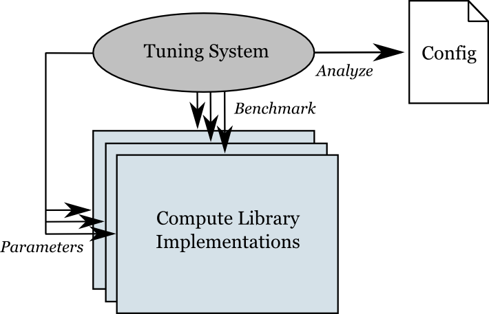
The purpose of the tuning system is to generate the configuration file rapptune.h that is needed when building the library. The tuning system does this by running a suite of benchmark tests, and analyzing the measured performance for each candidate implementation, as shown in figure 2.

Figure 2: The Tuning Process.

Overview

The tuning system consists of all files in the compute/tune and compute/tune/benchmark directories. It is layered on top of the standard build system. When needed, it is executed as part of e.g. make all. By separating the tuning system from the build system, the latter can be kept simple, and we can reuse it for the tuning purposes.

If the library is not already tuned, we add the tune directory to the SUBDIRS variable of compute/Makefile.am, to connect the tuning system to the ordinary build system. This effectively makes the build system re-entrant. That might seem like a contradiction to what was stated earlier about separation, but it is really only a matter of letting one system dispatch the other one. Their inner workings are still kept hidden from each other.

The Tuning Process

The tuning process consists of the following steps:

For each set of candidate options, create a separate build subdirectory and configure RAPP there, using the option --with-internal-tune-generation=CAND, where CAND has the form <impl>,<unroll>, specifying the implementation and unroll factor for the candidate. Besides causing various RAPP_FORCE flags to be set for the build, this internal option shortcuts those parts of RAPP that don't apply when tuning, for example stopping compute/tune from being used, and stopping re-generation of e.g. documentation. The parts that need to be aware of this re-entrancy are confined to the top-level configure.ac script and the compute/tune/Makefile.am file.
In each such subdirectory, build a library with the implementation candidates using the configured set of options. Configuration, building and installation for each candidate subdirectory will happen in parallel, if a parallel-capable make program such as GNU make and its -j option is used.
Install candidate libraries temporarily in the build directory archive as separate libraries, named rappcompute_tune_<impl>_<unroll>.
Build the benchmark application in compute/tune/benchmark.
Create a self-extracting archive rappmeasure.run, containing the library candidates, the benchmark application, the script compute/tune/measure.sh and the progress bar script compute/tune/progress.sh.
If we are cross-compiling, the user is asked to manually run rappmeasure.run on the target platform. Otherwise it will be executed automatically. When finished, it has produced a data file tunedata.py.
Run the analyzer script compute/tune/analyze.py on the data file. It creates the configuration header rapptune.h and a report tunereport.html.

After tuning, all the generated files are located in the compute/tune directory of the build tree. To make RAPP tuned for the platform for everyone else, they must be copied to the source directory and/or added to the distribution. A tarball to send to the maintainers, containing the necessary files, can be created using the make-target export-new-archfiles. There's also a make-target update-tune-cache to use for copying the generated tune-file and HTML report to the right place and name in the local source directory. Alternatively, together with benchmark HTML after benchmark tests, use the make-target update-archfiles.

Measuring Performance

The benchmark application takes the Compute layer library as an argument and loads it dynamically. It then runs its benchmark tests for the functions found in library, measuring the throughput in pixels/second. If a function is not found, the throughput is zero.

The script measure.sh runs the benchmark application with different library implementations and different image sizes. It generates a data file in Python format containing all measurement data.

Performance Metric

When the measurement data file is generated, the Python script analyze.py is used to analyze the data and determine the optimal implementations and parameters and generate the configuration header rapptune.h. To be able to compare the performance between two implementations, we need some sort of metric.

For a particular function, we can have several possible implementations. Order them from 1 to N, where N denotes the total number of implementations. For each implementation we also have several benchmark tests, corresponding to different image sizes. Let M denote the number of tests. For our function, we get an $M \times N$ matrix of measurements in pixels/second:

$\mathbf{P} = [ p_{ij} ].$

We want to compute a ranking number $ r_j $ for each implementation $ j $ of the function. First we compute the average throughput across all implementations:

$q_i = \frac{1}{N} \sum_{j=1}^{N} p_{ij}.$

Next, we normalize the data with this average value, creating a data set of dimensionless values,

$\hat{p}_{ij} = \frac{p_{ij}}{q_i}.$

These normalized numbers describe the speedup for a given implementation and test case, compared to the average performance of this test case. The normalized numbers are independent of the absolute throughput of each test case. This is what we want, since a fast test case could otherwise easily dwarf the results of the other tests. We want all test cases to contribute equally.

Finally, we compute the dimensionless ranking result as the arithmetic mean of the speedup results across all the test cases,

$r_j = \sqrt[M]{\prod_{i=1}^{M} \hat{p}_{ij}}.$

The implementation with the highest ranking gets picked and the parameters are written to the configuration header rapptune.h.

Tune Report

The analyze.py script also produces a bar plot of the tuning result in HTML format. It shows the relative speedup for the fastest one (any unroll factor) of the generic, SWAR and SIMD implementations. The gain factor reported is the ranking result, normalized with respect to the slowest bar plotted. Only functions with at least two different implementations are included in the plot.

Next section: Benchmark Tests