Magellan
A forward marine magnetic modeling program

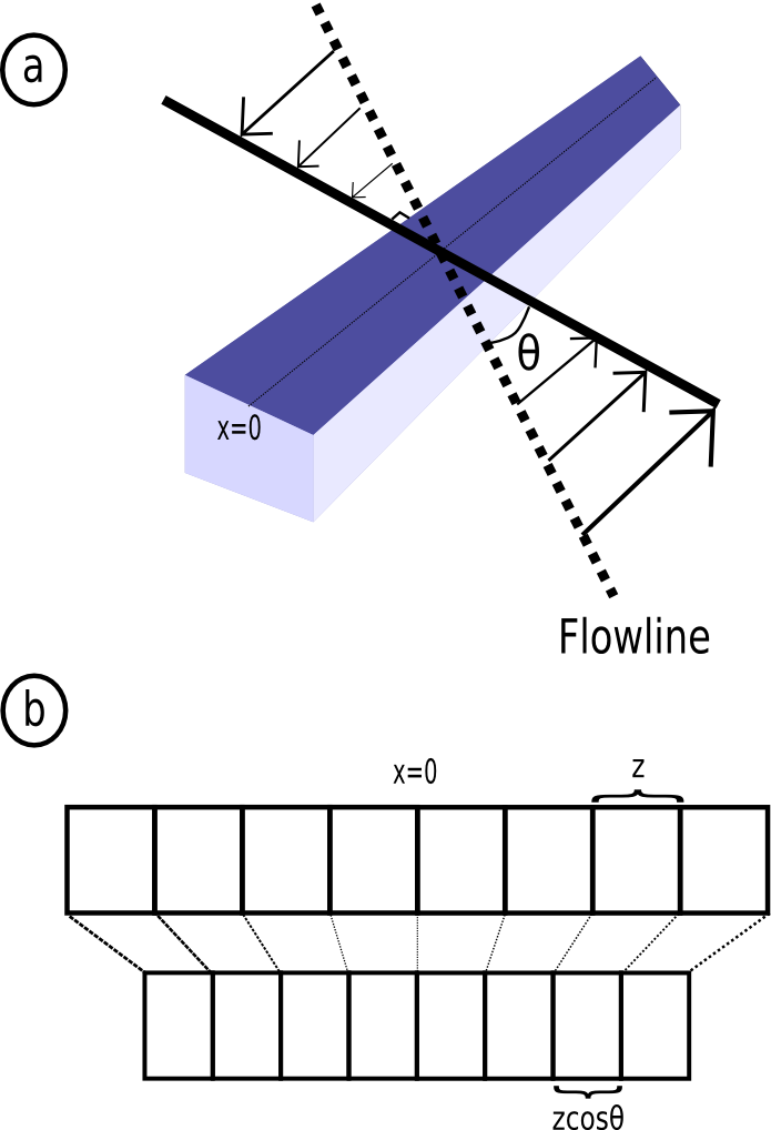
Oblique Spreading

When the magnetic model in Magellan is calculated the profile, along which the model is calculated, is assumed to run perpendicular to the strike of the ridge. This is true for most spreading centers in the world but where this is not true the assumption does not hold and the obliqueness of the spreading has to be taken into account.

Fig 1. Graphical explanation of the obliqueness problem. See text for details.

In Magellan a parameter called 'obliquity' is used to deal with this problem. The obliquity is the deviation from the orthogonal spreading and ranges from 0 to 90 degrees. Obliquity of 0 degrees represents an orthogonal spreading system. If the spreading direction of a ridge striking 120/300 degrees from north is 200/020 or 040/220 the obliquity is 10 degrees. Figure 1a demonstrates this. The dashed line is the flowline (200/020 or 040/220 in the example above) and the solid line runs perpendicular to the ridge (30/210 in the example above). The angle between the dashed and solid lines is the amount of obliquity to use (30-20=10, 220-210=10, etc. in the example above). Note that the cosine of the obliquity is used, not the obliquity directly, so the sign of the obliquity doesn't matter (cos(theta)=cos(-theta)).

To solve the obliquity problem the following procedure is performed
1. The magnetized blocks are arranged according to the input parameters (spreading rates, etc.) along the flowline of the ridge. This ensures that seafloor spreading is imitated correctly.
2. The magnetized blocks are projected perpendicular to the ridge. It is here where the cosine of the obliquity parameter is used. The width of the magnetized blocks is reduced by cos(theta), where theta is the obliquity angle. This is represented in Figure 1b. Note that the blocks are narrowed toward the ridge crest, which is different from the method of the contamination coefficient .
3. The magnetic model is calculated. In this situation the blocks are perpendicular to the ridge and thus the orthogonal spreading assumption is valid.
4. The magnetic model is projected back to the flowline and plotted along with the magnetized blocks, displayed with the correct width.