Conditional Operations

Introduction

When working with more complex analytics/vision algorithms, it is necessary to process only a selection of pixels. Typical applications use a cascade of algorithms. First, we start with simple algorithm that processes the entire image. It is fast but may produce many false positives. The parts of the image that pass this quick-rejection test move on to the next processing step, and so on. As we move up the ladder of algorithm complexity, the data processed becomes more and more sparse. There are two major problems with this:

Sparse data cannot be processed efficiently with SIMD technology.
Mixing arithmetic with conditional branching in the inner loop kills performance.

The gather/scatter mechanism of conditional processing aims to solve this issue.

The Gather/Scatter Mechanism

The gather/scatter mechanism is a generic framework for conditional pixel processing. It allows the user to

Increase performance on sparse images by not processing all pixels.
Alter a selection of pixels and leave the rest unchanged.
Leverage the power of SIMD-accelerated processing functions.

The basic concept is to decouple the selection of pixels from the actual processing. The gather and scatter functions handle this selection, while most of the other functions in this library do the processing.

The Theory of Gather and Scatter

Basic Definitions

We start by defining an ordering function for the coordinates in a two-dimensional image, $ r = r(x, y) $ . It has the following properties:

It is invertible.
It is strictly increasing in x, i.e. .

Define a function $[f_x, f_y] = f(\mathbf{m}, k)$ to be the x and y coordinates of the k:th non-zero ordered pixels in a binary map image m. Define h as

$h(\mathbf{m}, x, y) = \sum_{r(i,j) < r(x,y)} m_{ij},$

i.e. the sum of all ordered map pixels up to, but not including, the pixel at x, y. Finally, define n(m) as the sum of all pixels in the binary map:

$n(\mathbf{m}) = \sum_{ij} m_{ij}.$

Now we can define the gather function:

$G(\mathbf{u}, \mathbf{m}) = [u_{f(\mathbf{m}, 1)}, u_{f(\mathbf{m}, 2)}, \dots, u_{f(\mathbf{m}, n(\mathbf{m}))}],$

where u is an arbitrary w x h image. The dimension of G is 1 x n(m).

The gather function $ G $ is invertible for all non-zero pixels in the map. The scatter function is such an inverse in that sense:

$S(\mathbf{p}, \mathbf{m}) = [ m_{xy} p_{h(\mathbf{m},x,y)} ]_{xy},$

where p is an arbitrary 1 x n(m) vector.

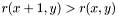
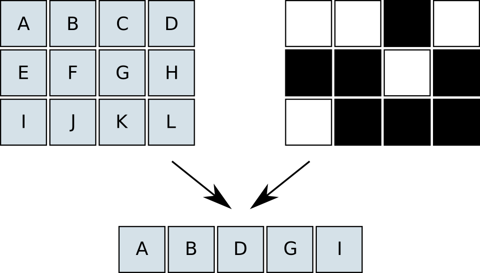
The gather function can be seen as compressing an w x h image into a 1 x n(m) image, with the map m as a key. The scatter function then restores the compressed pixels, using the same map. If our image processing is independent of the raster position and does not use any neighbouring pixels, we can perform the processing in the compressed domain. Examples of operations are pixelwise arithmetics, thresholding, pixel variance and histograms. Figures 1 and 2 illustrate the basic gather and scatter operations.

Figure 1: The Gather operation.

Figure 2: The Scatter operation.

Neighbourhood Access

The gather/scatter mechanism can be extended for use with operations that require a local neighbourhood of pixels, e.g. spatial filtering operations. We describe the technique for processing a 3x3 neighbourhood, but the concept holds for arbitrary window sizes.

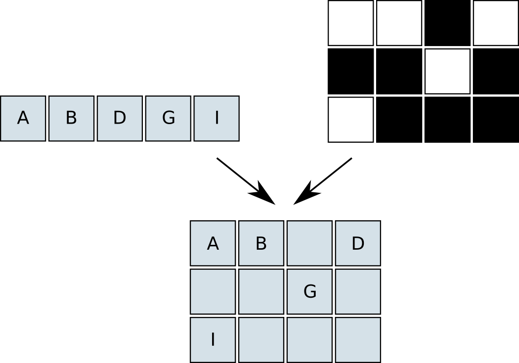
Let m₀ denote the binary map image. We dilate this map with a 1x3 structuring element, producing a new map m₁. This essentially pads the non-zero pixels in the horizontal direction. Next, we perform three gather operations with the dilated map, starting from the three top rows of the source image. We store the gathered data in three different rows in the pack image p of size 3 x n(m₁). For all pixels designated by the original binary map, the neighbours are available in the pack image on exactly the same relative positions as in the source image. We can now run our 3x3 spatial operations on the middle row of the pack image.

The processing of the pack image will produce correct results only for the original pixels of interest. If we scatter the 1 x n(m₁) result back to a destination image, also the invalid values for the pad pixel will be written. There are two ways to fix this problem:

Clear the pad pixels after scattering, using XOR of the map and the padded map.
Scatter only the relevant pixels.

The first alternative is probably best if the pixels to scatter are binary data, i.e. the processing ends in some threshold operation.

The second approach is more general. We create a residual map m₀₁ by gathering m₀ with m₁,

$\mathbf{m}_{01} = G(\mathbf{m}_0, \mathbf{m}_1).$

It is a map of the extra pixels that need to be gathered when translating gatherings with m₁ to m₀, i.e.

$G(\mathbf{u}, \mathbf{m}_0) = G(G(\mathbf{u}, \mathbf{m}_1), \mathbf{m}_{01}).$

With this map, we can gather the result pixels to a new, smaller pack buffer, and then scatter them to the destination image using the original map m₀. Figure 3 shows an example of the 3x3 processing.

Figure 3: A 3x3 neighbourhood example. Starting from the left on the first row, we have the source image u where the light blue pixels are the pixels of interest. The image m₀ is the map image, designating the the pixels of interest in the source image. First, we perform a 1x3 binary dilation on the map image, producing a new map m₁. Next, we perform three gathering operations with the map m₁, starting on the first three rows of the image u. The result is written to the three rows of the image p. Note how every blue pixel in the middle row are surrounded their 3x3 neighbours from the source image. On the image p we can now compute our 3x3 neighbourhood result for this middle row. It will be correct only for the blue pixels. To gather the correct result, we create the residual map **m₀₁** by gathering m₀ with m₁. The result of the 3x3 operation is then gathered by this map, producing the result in the last row. This is the correct result of the 3x3 operation on the original image, gathered by the original map m₀.

Performance

The performance gain of using the scatter/gather technique is highly dependent on the density of the map image and which operations are performed. For the basic scatter/gather use case, we get the saving in processing cost

$\Delta C = (w h - n) C_{proc} - C_{GS},$

where $C_{proc}$ is the per-pixel processing cost, $C_{GC}$ is the cost of the gather and scatter operations, n is the density of the binary map (number of non-zero pixels), and w, h is the image size.

It is obvious that the processing term will eventually dominate over the gather/scatter term as long as not all map pixels are set, given a high enough cost of processing. This is expected – the cost of gather and scatter will be amortized over the total processing performed in the compressed domain.

What is not obvious is that the cost of gather/scatter is also dependent on the map density n. If the map is sparse, the zero pixels in it will be discarded rapidly. However, this just alters the break-even threshold a bit, making it feasible to use the gather/scatter mechanism in cases of lightweight processing and sparse maps.

For the neighbourhood processing we get similar results. The map density of interest is now the density of the padded map.

Usage

In general, the cost saving is dependent on the cost of processing, and the layout of the map image in a non-trivial way. However, modelling it as a function of n is a reasonable approximation. The typical usage is as follows:

Compute the number of pixels in the map, using rapp_stat_sum_bin().
If the number of pixels is less than a constant threshold, perform gathering.
Perform the processing on either the full images, or the pack images.
Scatter the result if packed.

The threshold is processing and platform dependent, and must be set to a reasonable value by profiling the algorithm.

The gather/scatter mechanism can be used in cascade. This means that

The scattered binary output from one algorithm can serve as the map for the next algorithm in the chain.
If two cascaded algorithms use the same source data, it is not necessary to scatter the binary output of the first one back to the image domain. We can simply gather the compressed domain directly, which can cut the cost of the gather/scatter operations substantially.

Next section: Single Conditional Operations