
Contents:
Introduction
Overview
Mesh
Centering
A Note on Allocation
Geometry
A Note on Positions
Field
A Note on Allocation
Example: One-Dimensional Scalar Advection
Example: N-Dimensional Scalar Advection
Summary
As mentioned in an earlier tutorial, POOMA provides classes that know enough about their own spatial structure to manage stencil operations and the like automatically. The most important of these classes, Field, is the main subject of this tutorial. In order to understand how discrete Fields are built and used, however, it is necessary to understand how meshes are represented, what a centering is, and how DiscreteGeometry and related classes are used. After a quick overview of how these concepts tie together, this tutorial therefore describes POOMA's mesh abstraction, then its representation of centerings, then its geometry abstraction, and finally how the two are tied together by Field.
An array is a multi-element data structure, each of whose elements is specified by one or more indices. An array's indices don't mean anything in and of themselves; their only purpose is to order the array's elements.
A field, on the other hand, defines a set of values on a region of space. As with an array, the indices used to access a field's elements specify ordering and adjacency. Unlike an array's indices, however, a field's indices also have meaning: there is no "place" corresponding to element (2,2) of an array (except in a very abstract sense), but the third element of the third row of a field has some definite position in space.
In order to specify a field, a library such as POOMA must specify the locations at which the field's values are defined, and describe what happens at the boundaries of that region in space. The first of these tasks is handled in POOMA by geometry classes, which are used as template parameters to the Field class. This release of POOMA only provides geometry classes for discrete Fields; geometry classes capable of representing continuous Fields may be included in future releases. This release of POOMA further restricts all of its predefined geometry classes to represent discrete sets of points defined relative to a mesh, which is a set of connected points that spans a region of space. Meshes are discussed in the next section.
In addition to a mesh type, the geometry classes are parameterized by a centering type which describes the relationship of the geometry's points to the mesh. As discussed below, the points' locations relative to the mesh can, for example, be the mesh vertices, the cell centers, the face centers, or the edge centers. POOMA provides several classes to represent the mesh abstraction, several classes to represent the centering abstraction, and a DiscreteGeometry<Centering,Mesh> class which combines these to represent geometries. These are all described in detail later.
The second task of fields---describing what happens at the boundaries of a region of space---is handled in POOMA by boundary condition classes. So far, POOMA provides only predefined boundary condition classes for discrete Fields centered relative to logically rectilinear meshes. Various kinds of reflecting, constant, extrapolating, and periodic boundary conditions are supported.
Geometry and boundary-condition classes support the application-level Field class, which represents the field abstraction. Like an Array, a Field can be used in data-parallel expressions, subscripted with scalar indices and domains of various shapes and sizes, and so on. However, Fields also have an understanding of the spatial locations of their values, and of their boundary conditions. For example, the spatial locations of a Field's elements can be accessed using the member function Field::x().
A mesh is a discrete domain (i.e. a discrete set of points in coordinate space) and some kind of connectivity rule. This rule specifies which points in the mesh are connected to which others to form edges. In turn, sets of edges define faces, and sets of faces specify the boundaries of zones or cells in space.
POOMA contains a set of related classes to represent meshes. The classes in this release represent meshes which are logically rectilinear. They are not necessarily physically rectilinear because they support curvilinear as well as Cartesian coordinates. However, the template arguments, constructor parameters, and accessor methods of these classes allow for future releases to provide more general meshes, such as unstructured meshes with heterogeneous zones.
Like most POOMA classes, meshes can be constructed and initialized in two ways. The first technique is to pass parameters to a constructor to initialize the mesh's characteristics. The second is to construct the mesh using its default constructor, and then call its initialize() method with the parameters that would have been passed to a more complex constructor. (This second technique is typically used when allocating arrays of meshes.) All of POOMA's mesh classes provide a method called initialized(), which only returns true if the object has been fully initialized.
UniformRectilinearMesh is the simplest of POOMA's mesh classes. It represents a region of space that is divided at regular intervals along each axis (although the spacing along different axes may be different). In the 3-dimensional case, for example, the faces of a UniformRectilinearMesh are rectangles. Each zone is a block with six faces, and is dx×dy×dz in size, where dx, dy, and dz are the spacings along the mesh's three axes.
The RectilinearMesh class generalizes UniformRectilinearMesh by allowing the spacings to vary along each axis. This kind of mesh is sometimes called a Cartesian-product or tensor-product mesh. The divisions along each axis ai are defined by a set of intervals dai = {dai0, dai1, ..., daiN} (so that the jth interval on axis i has width daij). The whole mesh is then defined by the outer product da0×da1×...×daR-1 (where R is the rank of the mesh, i.e. the number of dimensions it has).
The template parameters for RectilinearMesh and UniformRectilinearMesh are identical, and both support the same basic set of constructors. The main difference between the two classes from a user's point of view is the extra constructors that RectilinearMesh provides. For clarity's sake, only the the two-dimensional constructors are shown below. Both classes define constructors which specify defaults for the origin and spacing; more constructors may be added in future releases.
template<int Dim,
         class CoordinateSystem = Cartesian<Dim>,
         class T = POOMA_DEFAULT_POSITION_TYPE>
class UniformRectilinearMesh
{
  template<class Dom1, class Dom2>
  UniformRectilinearMesh(const Dom1 &d1,
                         const Dom2 &d2,
			 PointType_t origin,
			 PointType_t spacings)
  {
    constructor body
  }

  rest of class
};

template<int Dim,
         class CoordinateSystem = Cartesian<Dim>,
         class T = POOMA_DEFAULT_POSITION_TYPE>
class RectilinearMesh
{
  template<class Dom1, class Dom2, class EngineTag>
  RectilinearMesh(const Dom1 &d1,
                  const Dom2 &d2,
		  const PointType_t &origin,
                  const Vector<Dim, Array<1, T, EngineTag > > &spacings,
                  const Vector<2*Dim, MeshBC> &mbc)
  {
    constructor body
  }

  rest of class
};
The Domi arguments to the constructors must be domains, and serve the same purpose as the domain constructor arguments used by the Array class. Only one argument is needed if that argument is a Dim-dimensional domain such as an Interval<Dim>. However, unlike Arrays, the domain must be zero-based, i.e. the origin of its index space must be [0,0,...0]. (This requirement may be relaxed in future versions of POOMA.) The spatial origin of each type of grid is specified by the constructor's origin parameter. UniformRectilinearMesh then takes another point, spacings, whose values specify the spacings along each axis.
The inter-element spacings for a RectilinearMesh, on the other hand, are specified using a Vector of one-dimensional Arrays. Such a structure can be defined and filled using code like the following:
Vector<D, Array<1,int> > spacings;
for (d = 0; d < D; d++) {
  spacings(d).initialize(cellDomain[d]);
  for (i = 0; i < cellDomain[d].size(); i++) {
    spacings(d)(i) = (i+1)*10;
  }
}
For RectilinearMesh, the mesh's boundary conditions are specified by giving an enumeration element for each face of the mesh (which is why there are twice as many boundary condition specifiers as mesh dimensions). The values allowed for the mesh boundary conditions in this release of POOMA, which are defined in src/Meshes/MeshBC.h, are LinearExtrapolate, Periodic, and Reflective. For UniformRectilinearMesh, the only sensible boundary condition is linear extrapolation (extension using the constant spacings below the origin and beyond the physical mesh upper boundary), which is built into the class; its constructors do not include MeshBC enum parameters.
Of course, before a set of points in space or spacings between them can sensibly be specified, a coordinate system must be chosen. This is the purpose of the CoordinateSystem template parameter. Its default value, Cartesian, produces a Cartesian (truly rectilinear) mesh. Other coordinate systems can also be used: Cylindrical, for example, produces a cylindrical coordinate system which is curvilinear. The discrete mesh, however, is indexable like a Cartesian mesh, i.e. it is still logically rectilinear.
In order to allow applications to operate on meshes without hard-coding the mesh's size, spacing, or coordinate system, the mesh classes store information about their domains in Array data members. (Where possible, these arrays are implemented using compute engines, so that memory is not wasted recording simple sequences of values.) Once accessed, these information arrays can be used in data-parallel expressions like any others. In particular, they are often used with stencils to implement differential operators such as div()and grad()(as discussed in the next tutorial).
The Arrays in POOMA's mesh classes have guard layers, which are extra elements outside their calculation domain whose values are defined by the mesh's boundary conditions. All of the mesh classes in this release automatically create guard layers that have ND/2 elements along each axis D, where ND is the number of vertices along that axis. This provides enough space for any plausible accesses to mesh data outside the mesh boundaries, such as locating the nearest vertex to a particle outside the boundary, or implementing a stencil operating on a Field centered at the mesh vertices which uses Field values at, and mesh spacings between, vertices beyond the boundary by a distance corresponding to the stencil width.
A mesh's positional data can be accessed using two pairs of public methods. physicalDomain() returns the mesh's physical domain (i.e. its vertex index domain), excluding its guard vertices. physicalCellDomain() returns a domain representing the mesh's cells; for a logically-rectilinear mesh, this is just one element smaller per dimension than physicalDomain() (since a rectilinear mesh has one fewer cells than vertices). Similarly, totalDomain() returns the domain of the mesh including its guard vertices, and totalCellDomain() performs a similar function for the mesh's cells. The methods vertexPositions() and vertexDeltas() access the mesh's vertices and spacings respectively. All these methods return references to Array data members, which can then be used like any other (read-only) Array.
A mesh does not fully specify the geometry of a discrete field until it is combined with a centering. Centerings are defined relative to the features that uniquely identify a mesh, such as its vertices, zones, faces, and edges. Figure 1 illustrates these features for an example mesh zone in one, two, and three dimensions.
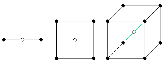 |
| Figure 1: Sample rectilinear mesh zones. Black circles are the vertices, and empty circles are the zone centers. The green axes help show that the zone center in 3D is in the physical center of the rectangular parallelepiped. |
The header file r2/src/Geometry/CenteringTags.h defines several classes which specify centerings in POOMA when used as template parameters to the DiscreteGeometry class discussed in the next section. The first two are non-template classes whose definitions are fairly simple:
struct Cell;
struct Vert;
For rectilinear meshes , these centering positions are just the white and black circles, respectively, from Figure 1.
The third predefined class in CenteringTags.h is a parameterized class specifically designed for logically rectilinear meshes, whose zones, vertices, faces, and edges can all be indexed in multi-dimensional array style (i.e. using (i,j,k)-style indices):
template <int Dim,
          class RectilinearCenteringTag,
          bool Componentwise = RectilinearCenteringTag::componentwise,
          int TensorRank     = RectilinearCenteringTag::tensorRank,
          int NComponents    = RectilinearCenteringTag::nComponents>
class RectilinearCentering
The RectilinearCenteringTag template parameter can be instantiated using a class whose centerings are defined componentwise. This means that each component of a multicomponent field element type such as Vector or Tensor can have its own independent centering position. The value of the Boolean template parameter Componentwise flags whether this is the case: if it is false, then all components of each multicomponent Field element are centered at the same point, rather than different points.
The TensorRank and NComponents parameters are required for componentwise centerings. TensorRank is the number of indices required to index a component of the multicomponent field element type, i.e. 1 for Vectors, and 2 for Tensors. NComponents is the number of values indexed by each component index, such as Dim for Vector<Dim> or Tensor<Dim>.
The actual descriptive information about the centering is in the RectilinearCenteringTag parameter. POOMA provides a set of classes and class templates that can be used as the RectilinearCenteringTag parameter:
// Centering on faces perpendicular to Direction:
template<int Direction>
class FaceRCTag;

// Centering on edges parallel to Direction:
template<int Direction>
class EdgeRCTag;

// Componentwise centering; each component centered on face perpendicular to
// that component's unit-vector direction:
template<int Dim>
class VectorFaceRCTag;

// Componentwise centering; each component centered on face parallel to that
// component's unit-vector direction:
template<int Dim>
class VectorEdgeRCTag;
As an example, the FaceRCTag in three dimensions defines centering points on the zones' rectangular face centers, perpendicular to the direction specified by the template parameter. With Direction=0 (the X direction), this defines the face centers perpendicular to the X axis. In two dimensions, zone faces and zone edges are degenerate; in one dimension, faces are further degenerate with vertices. Figure 2 shows the FaceRCTag<0> centering positions (red circles) relative to a single zone in these cases.
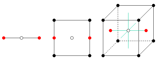 |
| Figure 2: Centering positions of FaceRCTag<0> in 1, 2, and 3 dimensions. |
Figure 3 shows an example two-dimensional mesh with 4×4 vertices (and thus 3×3 cells), with the complete set of FaceRCTag<0> centering points shown. Note that it is really the geometry class using the centering class that determines where the coordinate locations of the centering points are; the figure shows the standard definition (i.e. the geometric centers of the faces). Note also that the number of centering points is equal to the number of cells in the Y direction and the number of vertices in the X direction. A geometry class using this centering would provide centering position vectors indexable on this physical indexing domain.
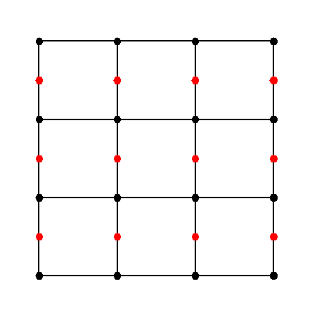 |
| Figure 3: Two-dimensional mesh with complete set of centering points. |
As an example of componentwise centering, consider RectilinearCentering<2,VectorFaceRCTag<2> >. The Y components of a field element of Vector type are centered on the faces perpendicular to the Y axis, while the X components are centered on the faces perpendicular to X. Figure 4 illustrates this, by showing the X and Y components as horizontal and vertical arrows rooted at their centering points. The dotted blue lines indicate which pairs of components are components of a single field element. The green arrows indicate valid X and Y components at the extremal high-end faces. It is only legal to refer to the one valid component of a vector at this location (using its corresponding IJK index). The companion perpendicular components for these values are not defined. (See the note on allocation below for more details.)
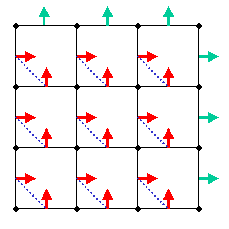 |
| Figure 4: Example of componentwise centering, showing RectilinearCentering<2,VectorFace<2>> |
For componentwise rectilinear centerings such as RectilinearCentering<2,VectorFace<2> >, POOMA currently allocates Field domains (and Array domains in the associated DiscreteGeometry) with storage for nVerts elements in each dimension, so storage for a Vector with both components at these extremal locations is allocated, but only the valid component is legally accessible.
The next layer of support in POOMA for fields is its geometry abstraction. A geometry is a set of points in a coordinate space. This implies a definition of a coordinate system, an explicit or implicit specification of the points in the set, and what if any boundaries bound the set of points. A geometry might be a continuous set of points, but currently POOMA only provides geometry classes to represent discrete sets of points. Furthermore, POOMA's current geometry classes are restricted to sets of points defined relative to a mesh (represented by one of the POOMA mesh classes described above) according to a centering (represented by one of the POOMA centering classes described above).
Geometries are described in this release of POOMA by partial specializations of the DiscreteGeometry class template. DiscreteGeometry itself is defined in src/Geometry/DiscreteGeometry.h. The class has an empty body (i.e. no methods or data members), and is parameterized as:
template<class Centering, class Mesh> class DiscreteGeometry;
The two header files DiscreteGeometry.URM.h and DiscreteGeometry.RM.h instantiate this class with particular template parameters to create the UniformRectilinearMesh and RectilinearMesh classes respectively. Both of these classes inherit from the RectilinearGeometryBase class, which among other things defines default implementations for DiscreteGeometry's x(), totalDomain(), and physicalDomain() methods. Field relies on these to implement its own methods---for example, Field::x() simply forwards its arguments to its geometry data member, on the assumption that this member will itself have a method called x().
By default, a POOMA geometry does not have any guard cells, i.e. its total domain is the same as its physical domain. (See the section on meshes for an explanation of these terms.) An application can request guard layers for a geometry by passing a GuardLayers object to the geometry's constructor, or equivalently its initialize() method. GuardLayers is defined in src/Layout/GuardLayers.h, and simply describes the depth of the guard layer along each axis.
POOMA's geometry abstraction describes a set of points in space, and is intended to serve primarily as a domain (in the functional sense) of something like a field. In order to be used in this way, i.e. in order to be used as the Geometry template parameter to POOMA's Field class, a class must define certain constants, types, and methods. The two required constants are:
The types which a geometry class must define are:
PositionArray_t is the type of Array object "storing" the geometry's set of position values. For the DiscreteGeometry types based on rectilinear meshes provided in this release of POOMA (i.e. those whose Mesh template parameter is UniformRectilinearMesh<Dim> or RectilinearMesh<Dim>), PositionArray_t is an Array<Dim,PointType_t,PositionFunctor_t>. For a continuous geometry, this would be some kind of continuous Array type.
The array domain of that Array has type Domain_t. Domain_t must be a type which can serve as a constructor argument for that POOMA Array, and must have appropriate dimensionality. For the DiscreteGeometry classes mentioned in the previous paragraph, Domain_t is a typedef for Interval<Dim>. For a continuous geometry, it would be some object representing a continuous domain, like a sphere or a spline-surface-bounded solid.
Finally, a class which is to be used as a geometry must define the following methods:
The DiscreteGeometry-based classes provided with this release of POOMA actually provide a richer interface than the one described above. First, each of these classes defines the following constant:
Second, POOMA's DiscreteGeometry-based classes create the following convenience typenames:
Finally, the classes based on DiscreteGeometry define the methods listed below.
The class used as the Geometry template parameter for Field must provide methods for returning the spatial positions of its points. All of these methods in the geometry classes in this release of POOMA are based on Arrays of position Vectors which use compute engines. As an example, the DiscreteGeometry<Cell,Mesh_t> classes define the locations of the zone centers relative to the set of faces that define a zone. For logically rectilinear meshes, this is typically defined as the geometric center of the zone (which is what DiscreteGeometry<Cell,Mesh_t> defines it as), but this is not necessarily the case. A user could, for example, define a geometry class which used a UniformRectilinear or Rectilinear mesh, but which offset the definition of the zone centers from the geometric centers to implement special types of differential operators.
As stated above, the class Field represents both a region of space, and a set of values defined on and around that region---a mapping from points in the region to values. This release of POOMA only supports fields with up to three dimensions, although future releases of the library may support higher-dimensional structures.
Field has three template parameters. The first, Geometry, defines the region of space. The second and third template parameters to Field are like those of Array: they specify the type T of the field's values, and the type of the engine used for storing or evaluating the field's values. The whole definition is therefore:
template<class Geometry,
         class T = POOMA_DEFAULT_ELEMENT_TYPE,
         class EngineTag = POOMA_DEFAULT_ENGINE_TYPE>
class Field : parent classes
{
  body
};
A ConstField class with the same template parameters is also defined, just as a ConstArray is defined to accompany Array.
A Field has a value of type T at every point in the spatial domain defined by its geometry class parameter Geometry. In this sense, a Field is a concrete representation of a function, whose domain is specified by its geometry, and whose range is the set of values the Field contains.
A Field's values can be accessed or modified by subscripting the Field with scalar indices or an integer-based indexing domain such as an Interval (like an Array's values are accessed or modified). As well as storing values, a Field can provide information about the space on which it is defined. If f is a Field, then f.x() is a ConstArray with the same number of dimensions as f, whose elements are the positions at which f is defined. In one dimension, f.x(0) is therefore the position of one corner of the physical domain the Field represents; in functional terms, the field maps the point f.x(0) to the value f(0).
As mentioned above, this release of POOMA only supports discrete fields on regularly-spaced points in up to three dimensions. This restriction may be relaxed in future versions; in particular, continuous geometries and fields may also be supported. In this case, f.x() would return a continuous ConstArray, which would be accessed using floating-point indices, and which would use some analytic or interpolative function to return values.
The discussion of geometry above has implied the possible existence of layers of guard elements lying around discrete fields. These elements are used to implement boundary conditions, so that discrete operators can treat the "interesting" (i.e. interior) elements of Fields uniformly. A Field can automatically update parts of its domain using boundary condition objects stored in a list. Before being accessed, these boundary condition objects can be queried as to whether the domain they manage needs updating, and then told to update themselves if necessary.
POOMA predefines boundary-condition classes for use with Fields that are based on its rectilinear mesh geometry classes. The current release provides periodic, reflecting, constant, and linear-extrapolation boundary condition types; future releases may include others. More importantly, the required interface for the boundary condition classes is meant to make it easy for users to implement their own special boundary conditions. By following this interface prescription, applications can attach their own boundary conditions to Field objects and have them updated automatically, just as the predefined POOMA boundary conditions are updated. The interface allows writing boundary conditions using high-level array-syntax coding. (See the next tutorial for more information on writing boundary conditions in POOMA.)
Operations on Fields with global guard layers might need to access Field::x() positional values in those guard layers, for example to implement spatially-dependent boundary conditions, or to implement differential operators. Because of this, the geometry classes which Field uses must be able to supply positional values beyond the physical centering positions associated with the Fields' physical domain. This, in turn, means that the mesh classes used by discrete geometry classes need to return arrays of vertex positions beyond the edge of the actual mesh boundary, from which the geometry can compute the associated cell and face positions at which the Field is defined.
As discussed above, POOMA's mesh classes add guard layers to their contained arrays of positions, spacings, and volumes by making use of the fact that the indexing domain of an Array can start some number of elements below zero and extend beyond the number of vertices at the other side. The existence of guard layers affects the information that Fields provide about the spatial position of their elements. The expression f.x(0) is actually the position of one corner of the total domain of the Field f only if f has no guard layers, since the rule is that the physical domain of a Field is always zero-based. This means that in the presence of guard layers the actual corners of the Field will have negative indices. However, it is always true that the Field maps the point f.x(0) to the value f(0).
The number of guard layers in the DiscreteGeometry objects is determined by user input on construction (using GuardLayers<Dim> objects), and becomes the number of guard layers that the Field itself has as well. The DiscreteGeometry uses values from the guard layers in the mesh to fill its arrays of centering-point values (which are returned by its x() method). The number of guard layers specified for the DiscreteGeometry, and hence for any Field that is constructed using the DiscreteGeometry object, cannot be larger than the N/2 number of guard layers automatically defined in the RectilinearMesh or UniformRectilinearMesh object used to construct the DiscreteGeometry.
What's going on under the hood when an application makes a DiscreteGeometry object with this VectorFace type of componentwise centering for its Centering parameter? The DiscreteGeometry::totalDomain() method returns a domain with an extent of nVerts×nVerts×nVerts (in three dimensions). When the application constructs a Field using a geometry object as a constructor argument, it uses DiscreteGeometry::totalDomain() in order to allocate its own Array storage. The geometry classes have internal Array data members called positions_m which store the position values accessed by DiscreteGeometry::x(); in all the existing DiscreteGeometry partial specializations, these Arrays have compute-based engines, so they don't allocate any storage.
The domains of these Arrays must still be specified. In a geometry class which has VectorFace for its Centering template parameter, these compute-based Array data members have their domains set to nVerts×nVerts×nVerts. Any Field which uses this geometry (whose Field::x() method forwards to Field::geometry()::x()) will therefore automatically have its domain aligned with that of the geometry.
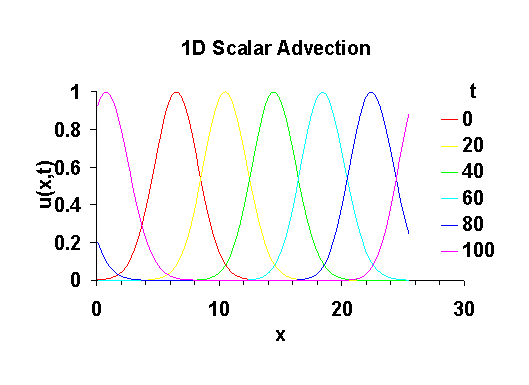
The example program in examples/Field/ScalarAdvection1D illustrates the features of fields introduced so far by simulating advection in one dimension. A later example in this tutorial shows how to generalize this to handle N dimensions.
The partial differential equation involved is:
where v is a constant propagation speed, and da/db represents the partial derivative of a with respect to b. The analytic solution of this is just a rightwards propagation at speed v of the initial condition:
The figure below shows that the numerical solution approximates this well.
This equation is a special 1-dimensional version of the general flux-conservative equation:
where F is a vector function:
The N-dimensional scalar advection program discussed later solves this equation for the special case where Fx = vx*u, Fy = vy*u, and Fz = vz*u. Note that in one dimension this reduces to exactly the 1D PDE stated above.
The one-dimensional code is shown below. For this particular differential equation, a simple Euler scheme is unstable, so the code uses a leap-frog method based on the difference equation:
| (ujn+1 - ujn-1) / (2 dt) | = | - v (uj+1n - uj-1n) / (2 dx) |
This scheme is primed by executing a single Euler step:
| (ujn+1 - ujn) / dt | = | - v (uj+1n - uj-1n) / (2 dx) |
001  #include "Pooma/Fields.h"
002
003  #include <iostream>
004  using namespace std;
005
006  int main(int argc, char *argv[])
007  {
008    Pooma::initialize(argc,argv);
009
010    // Create the physical domains (1D):
011    const int nVerts = 129;
012    const int nCells = nVerts - 1;
013    Interval<1> vertexDomain(nVerts);
014
015    // Create the (uniform, logically rectilinear) mesh:
016    const Vector<1> origin(0.0), spacings(0.2);
017    typedef UniformRectilinearMesh<1> Mesh_t;
018    Mesh_t mesh(vertexDomain, origin, spacings);
019
020    // Create two geometry objects - one allowing 1 guard layer to
021    // account for stencil width and another with no guard layers to support
022    // temporaries:
023    typedef DiscreteGeometry<Cell, UniformRectilinearMesh<1> > Geometry_t ;
024    Geometry_t geom1c(mesh, GuardLayers<1>(1));
025    Geometry_t geom1ng(mesh);
026
027    // Create the Fields:
028
029    // The flow Field u(x,t):
030    Field<Geometry_t> u(geom1c);
031    // The same, stored at the previous timestep for staggered leapfrog
032    // plus a useful temporary:
033    Field<Geometry_t> uPrev(geom1ng), uTemp(geom1ng);
034
035    // Initialize flow Field to zero everywhere, even global guard layers:
036    u.all() = 0.0;
037
038    // Set up Periodic Face boundary conditions:
039    u.addBoundaryCondition(PeriodicFaceBC(0));     // Low X face
040    u.addBoundaryCondition(PeriodicFaceBC(1));     // High X face
041
042    // Used various places below:
043    Interval<1> pd = u.physicalDomain();
044
045    // Load initial condition u(x,0), a pulse centered around nCells/4 and
046    // decaying to zero away from nCells/4 both directions, with a height of 1.0,
047    // with a half-width of nCells/8:
048    const double pulseWidth = spacings(0)*nCells/8;
049    const double u0 = u.x(nCells/4)(0);
050    u = 1.0*exp(-pow2(u.xComp(0)(pd)-u0)/(2.0*pulseWidth));
051
052    // Output the initial field:
053    std::cout << "Time = 0:\n";
054    std::cout << u << std::endl;
055
056    const double v = 0.2;  // Propagation velocity
057    const double dt = 0.1; // Timestep
058
059    // Prime the leapfrog by setting the field at the previous timestep
060    // using the initial conditions:
061    uPrev = u;
062
063    // Do a preliminary timestep using forward Euler, coded directly using
064    // data-parallel syntax:
065    u -= 0.5*v*dt*(u(pd+1)-u(pd-1))/spacings(0);
066
067    // Now use staggered leapfrog (second-order) for the remainder of the
068    // timesteps:
069    for (int timestep = 2; timestep <= 1000; timestep++)
070    {
071      uTemp = u;
072      u = uPrev-v*dt*(u(pd+1)-u(pd-1))/spacings(0);
073      if ((timestep % 200) == 0)
074      {
075        // Output the field at the current timestep:
076        std::cout << "Time = " << timestep*dt << ":\n";
077        std::cout << u << std::endl;
078      }
079      uPrev = uTemp;
080    }
081
082    Pooma::finalize();
083    return 0;
084  }
After initializing the POOMA library, this code sets up the world on which the equation is to be solved. Lines 11-13 define the size of the simulation, while lines 16-18 define the mesh on which calculations will be performed. Lines 23-25 then use this mesh to define two geometry objects. The first, geom1c, includes a guard layer, so that a finite difference stencil can be applied safely. The second, geom1ng, does not include this guard layer, but instead only represents the "actual" region of the solution. This geometry is used to define temporaries, as discussed below.
The actual flow field variable u is declared on line 30. Since this is the variable to which the full stencil is later applied, it uses the full geometry geom1c (the one with the guard layer). The Field used to record the previous iteration's results, and a general-purpose temporary, are declared on line 33. These Fields use the geom1ng geometry, which does not include memory for guard layers. While the memory saved by not having guard layers for temporaries is insignificant in this case, it can be substantial on larger problems, and in more dimensions.
The field u is initialized to zero everywhere (even in its guard layers) on line 36, using the method all() to get a reference to the whole of the field's data. Periodic boundary conditions are then set on lines 39-40. Line 43 then records the bounds on the problem domain in the Interval pd.
The statements on lines 48-50 insert a symmetric pulse into the field. The boundary conditions are applied after this is done to ensure that the field is in a consistent state. The values of the field at this point are then printed out, for later conversion into the graph shown earlier.
The constants controlling the simulation are set on lines 56-57, while the advection calculation itself is initialized on lines 61 and 65. The timestep is 0.1, and the propagation velocity is fixed at 0.2 (both in arbitrary units). After storing the initial state of the field in uPrev, so that the loop beginning on line 69 will perform its first iteration correctly, the program calculates the first set of new values for the field directly. Note how the domain of this calculation is defined using the pd value that was obtained from the field itself. This idiom helps ensure the consistency of large programs, which many juxtapose many different domains. It also helps make the program more robust in the face of incremental evolution: if the declaration of an important variable (like the Field u) is altered, calculations involving that variable reflect those alterations automatically.
The loop on lines 69-80 repeatedly updates the Field by invoking the calculation on line 72. The bulk of the code in the loop (lines 73-78) simply outputs the state of the Field every 200 iterations, so that a graph showing its evolution can be created later. Finally, the library is shut down, and the program terminated, on lines 82-83.
The most important thing to note about this program is the way in which various calculation domains are declared and combined. As a general rule, only a small number of calculation domains are ever declared from scratch; all others are then derived from these. As a corollary, the extent of calculations on Fields are usually determined by interrogating the Field, rather than by using long-lived Ranges or other objects. This helps keep the code correct as it evolves, and is also an important step toward generalizing codes such as this to handle an arbitrary number of dimensions.
The differential equation solved in the preceding example is a special 1-dimensional version of the general flux-conservative equation:
where F is a vector function:
The N-dimensional scalar advection program discussed in this tutorial solves this equation for the special case where Fx = vx*u, Fy = vy*u, and Fz = vz*u. Note that in one dimension this reduces to the equation shown in the previous example.
The N-dimensional code shown below revisits the scalar advection code shown earlier, using a less dimension-dependent implementation strategy. Again, since a simple Euler scheme is unstable for this particular differential equation, the code uses a leap-frog method based on the difference equation:
| (uijkn+1 - uijkn-1) / (2 dt) | = | - div(v uijkn) |
where:
in three dimensions, and the div() difference operator on the right-hand side is centered in space about (i,j,k), so that it involves differences of the form:
As described in the next tutorial, this is exactly what POOMA's div() function does, so the leap-frog timestepping is implemented using:
| u | = | uPrev - 2 div<Cell>(v dt u) |
This scheme is primed by executing a single Euler step, which also uses POOMA's div() function to do the space-centered differencing on the right-hand side:
| (ujn+1 - ujn) / dt | = | - div(v uijkn) |
| u | = | u - div<Cell>(v dt u) |
As we have seen, all of the important classes in POOMA take the dimension of the problem space as a template parameter. Provided all definitions in the program are made in terms of this parameter, or in terms of types exported from POOMA classes by typedefs, applications can move from two to three dimensions simply by changing line 13 in the following source code:
001  #include "Pooma/Fields.h"
002
003  #include <iostream>
004
005  int main(int argc, char *argv[])
006  {
007    // Set up the library
008    Pooma::initialize(argc,argv);
009
010    // Create the physical domains:
011
012    // Set the dimensionality:
013    const int Dim    = 2;
014    const int nVerts = 129;
015    const int nCells = nVerts - 1;
016    Interval<Dim> vertexDomain;
017    int d;
018    for (d = 0; d < Dim; d++)
019    {
020      vertexDomain[d] = Interval<1>(nVerts);
021    }
022
023    // Create the (uniform, logically rectilinear) mesh.
024    Vector<Dim> origin(0.0), spacings(0.2);
025    typedef UniformRectilinearMesh<Dim> Mesh_t;
026    Mesh_t mesh(vertexDomain, origin, spacings);
027
028    // Create two geometry objects - one allowing 1 guard layer to account for
029    // stencil width and another with no guard layers to support temporaries:
030    typedef DiscreteGeometry<Cell, UniformRectilinearMesh<Dim> > Geometry_t;
031    Geometry_t geom(mesh, GuardLayers<Dim>(1));
032    Geometry_t geomNG(mesh);
033
034    // Create the Fields:
035
036    // The flow Field u(x,t):
037    Field<Geometry_t> u(geom);
038    // The same, stored at the previous timestep for staggered leapfrog
039    // plus a useful temporary:
040    Field<Geometry_t> uPrev(geomNG), uTemp(geomNG);
041
042    // Initialize Fields to zero everywhere, even global guard layers:
043    u.all() = 0.0;
044
045    // Set up periodic boundary conditions on all mesh faces:
046    u.addBoundaryConditions(AllPeriodicFaceBC());
047
048    // Load initial condition u(x,0), a symmetric pulse centered around nCells/4
049    // and decaying to zero away from nCells/4 all directions, with a height of
050    // 1.0, with a half-width of nCells/8:
051    const double pulseWidth = spacings(0)*nCells/8;
052    Loc<Dim> pulseCenter;
053    for (d = 0; d < Dim; d++) { pulseCenter[d] = Loc<1>(nCells/4); }
054    Vector<Dim> u0 = u.x(pulseCenter);
055    u = 1.0 * exp(-dot(u.x() - u0, u.x() - u0) / (2.0 * pulseWidth));
056
057    // Output the initial field:
058    std::cout << "Time = 0:\n";
059    std::cout << u << std::endl;
060
061    const Vector<Dim> v(0.2);   // Propagation velocity
062    const double dt = 0.1;      // Timestep
063
064    // Prime the leapfrog by setting the field at the previous timestep using the
065    // initial conditions:
066    uPrev = u;
067
068    // Do a preliminary timestep using forward Euler, using the canned POOMA
069    // stencil-based divergence operator div() for the spatial difference:
070    u -= div<Cell>(v * dt * u);
071
072    // Now use staggered leapfrog (second-order) for the remaining timesteps
073    // The spatial derivative is just the second-order finite difference in the
074    // canned POOMA stencil-based divergence operator div():
075    for (int timestep = 2; timestep <= 1000; timestep++)
076    {
077      uTemp = u;
078      u = uPrev - 2.0 * div<Cell>(v * dt * u);
079      if ((timestep % 100) == 0)
080      {
081        // Output the field at the current timestep:
082        std::cout << "Time = " << timestep*dt << ":\n";
083        std::cout << u << std::endl;
084      }
085      uPrev = uTemp;
086    }
087
088    Pooma::finalize();
089    return 0;
090  }
The key lines are 13-15, which define the dimensionality of the simulation, and the size of the domain on which the simulation will be performed. Lines 18-21 then initialize an array of vertex domain objects, the number of elements in which is defined in terms of the Dim constant. Similarly, lines 24-32 create a mesh, and a geometry, in a dimension-independent way. Note that when a single value is passed to the constructor of an N-dimensional Vector, that value is assigned to all of the vector's elements. Note also the use of the vector dot product dot(Vector<>,Vector<>) in line 55 to compute the distance from the pulse-center point.
The rest of this program continues in this vein---periodic boundary conditions are set on line 46, for example, and the initial pulse is created on lines 51-55. The result is a program which is only six lines longer than its one-dimensional equivalent, but capable of changing dimension with ease.
One of the principal motivations behind POOMA is to provide C++
classes which directly address numerical science problems using the
language of numerical scientists. The Field classes
described in this tutorial exemplify this. By managing boundary
conditions, and supporting efficient evaluation of differential
operators, these classes provide the functionality that modern
numerical algorithms require, and allow numerical scientists to
concentrate on what they want to calculate, rather than on how it is
to be calculated.
| [Prev] | [Home] | [Next] |