
Contents:
Introduction
Particle/Field Interpolation
Laying Out Particles and Fields
Example: Particle-in-Cell Simulation
Summary
The previous tutorials have described how POOMA represents fields and particles. This tutorial shows how the two can be combined to create complete simulations of complex physical systems. The first section describes how POOMA interpolates values when gathering and scattering field and particle data. This is followed by a look at the in's and out's of layout, and a medium-sized example that illustrates how these ideas fit together.
POOMA's Particles class is designed to be used in conjunction with its Fields. Interpolators are the glue that bind these together, by specifying how to calculate field values at particle (or other) locations that don't happen to lie exactly on mesh points.
Interpolators are used to gather values to specific positions in a field's spatial domain from nearby field elements, or to scatter values from such positions into the field. The interpolation stencil describes how values are translated between field element locations and arbitrary points in space. An example of using this kind of interpolation is particle-in-cell (PIC) simulations, in which charged particles move through a discretized domain. The particle interactions are determined by scattering the particle charge density into a field, solving for the self-consistent electric field, and gathering that field back to the particle positions. The last example in this tutorial describes a simulation of this kind.
POOMA currently offers three types of interpolation stencils: nearest grid point (NGP), cloud-in-cell (CIC), and subtracted dipole scheme (SUDS). NGP is a zeroth-order interpolation that gathers from or scatters to the field element nearest the specified location. CIC is a first-order scheme that performs linear weighting among the 2D field elements nearest the point in D-dimensional space. SUDS is also first-order, but it uses just the nearest field element and its two neighbors along each dimension, so it is only a 7-point stencil in three dimensions. Other types of interpolation schemes can be added in a straightforward manner.
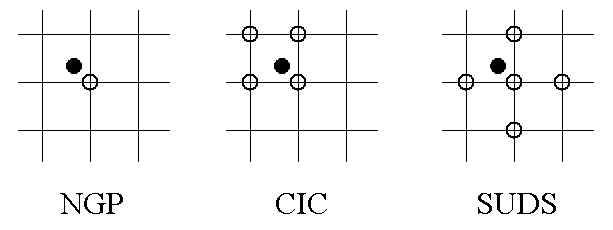 |
| Figure 1: Interpolation strategies. Black dots show particle positions, and open circles are the interpolation stencil points. |
Interpolation is invoked by calling the global functions gather() and scatter(), both of which take four arguments:
An example of this is:
gather(P.efd, Efield, P.pos, CIC());
where P is a Particles subclass object whose attributes are efd for storing the gathered electric field from the Field Efield and pos for the particle positions. The default constructor of the interpolator CIC is used to create a temporary instance of the class to pass to gather(), telling it which interpolation scheme to use.
The particle attribute and position arguments passed to gather() and scatter() should have the same layout, and the positions must refer to the geometry of the Field being used. The interpolator will compute the required interpolated values for the particles on each patch. These functions assume each particle is only interacting with field elements in the Field patch that exactly corresponds to the particle patch. Thus, applications must use the SpatialLayout particle layout strategy and make sure that the Field has enough guard layers to accommodate the interpolation stencil.
In addition to the basic gather() and scatter() functions, POOMA offers some variants that optimize other common operations. The first of these, scatterValue(), scatters a single value into a Field rather than a particle attribute with different values for each particle. Its first argument is a single value with a type that is compatible with the Field element type.
The other three optimized methods are gatherCache(), scatterCache(), and scatterValueCache(). Each of these has two overloaded variants, which allow applications to cache and reuse interpolated data, such as the nearest grid point for each particle and the distance from the particle's position to that grid point. The difference between the elements of each overloaded pair of methods is that one takes both a particle position attribute and a particle interpolator cache attribute among its arguments, while the other takes only the cache attribute. When the first of these is called, it caches position information in the provided cache attribute. When the second is called with that cache attribute as an argument, it re-uses that information. This can speed up computation considerably, but it is important to note that applications can only do this safely when the particle positions are guaranteed not to have changed since the last interpolation.
The use of particles and fields together in a single application brings up some issues regarding layout that do not arise when either is used on its own. There are two characteristics of Engines that must be considered in order to determine whether they can be used for attributes in Particles objects:
1. Can the engine use a layout that is "shared" among several engines of the same category, such that the size and layout of the engine is synchronized with the other engines using the layout? If this is the case, then creation, destruction, repartitioning, and other operations are done for all the shared engines. Particles require all their attributes to use a shared layout, so only engines that use a shared layout can be used for particle attributes. The only engines with this capability in this release of POOMA (i.e., the only engines that are usable in Particles attributes) are SharedBrick (using a SharedDomainLayout layout) and some specializations of MultiPatch.
MultiPatch can use several different types of layouts and single-block engines, and all MultiPatchs use a shared layout. However, only the MultiPatch<GridTag,*> types of MultiPatch engines are useful for Particles attributes, since only that engine type can have patches of varying size. Future releases of POOMA will add other layouts, such as TileLayout, that will also be useful for attributes.
Note that MultiPatch<UniformTag,Brick> can not be used for particle attributes, as it uses a UniformGridLayout. While that layout is "shared", UniformGridLayout is not useful for particles because it requires all patches to have the same size, and particle attribute patches change their size dynamically.
2. How many patches can the engine have? A SharedBrick can only have one patch, but a Grid-based MultiPatch can have several patches. Either one can be used in serial or in parallel, but their efficiency will differ. If individual particle attribute expressions will normally be run in parallel, the application should use a MultiPatch. Otherwise, it should use a SharedBrick.
Implicit in the discussion above is the fact that there are actually three different types of layout classes that an application programmer must keep in mind:
The only thing that needs to match between the attribute and Field layouts is the number of patches, which must be the same. The engine type (and thus the layout type) of the attributes and of the field do not have to match. An application could therefore use a SharedBrick engine for particle attributes, and a MultiPatch<UniformTag,Brick> for the Field, as long as the MultiPatch engine uses just one patch (since SharedBrick can only have one patch).
Note once again that in the simple case of a UniformLayout, applications do not need to worry about the Field layout type, only the particle attributes' layout (which still needs to be shared) and the particle layout (in this case, UniformLayout). This commonly arises during the prototyping (i.e., pre-parallel) stages of application development.
Our third and final example of this important class is a particle-in-cell program, which simulates the motion of charged particles in a static sinusoidal electrical field in two dimensions. This example brings together the Field classes of the preceding tutorials with this tutorial's Particles class.
Because this example is longer than the others in these tutorials, it will be described in sections. For a unified listing of the source code, please see the file examples/Particles/PIC2d/PIC2d.cpp in the distribution.
The first step is to include all of the usual header files:
001  #include "Pooma/Particles.h"
002  #include "Pooma/DynamicArrays.h"
003  #include "Pooma/Fields.h"
004  #include "Utilities/Inform.h"
005  #include <iostream>
006  #include <stdlib.h>
007  #include <math.h>
Once this has been done, the application can define a traits class for the Particles object it is going to create. As always, this contains typedefs for AttributeEngineTag_t and ParticleLayout_t. The traits class for this example also includes an application-specific typedef called InterpolatorTag_t, for reasons discussed below.
008  template <class EngineTag, class Centering, class MeshType, class FL,
009            class InterpolatorTag>
010  struct PTraits
011  {
012    // The type of engine to use in the attributes
013    typedef EngineTag AttributeEngineTag_t;
014
015    // The type of particle layout to use
016    typedef SpatialLayout<DiscreteGeometry<Centering,MeshType>,FL>
017      ParticleLayout_t;
018
019    // The type of interpolator to use
020    typedef InterpolatorTag InterpolatorTag_t;
021  };
The interpolator tag type is included in the traits class because an application might want the Particles-derived to provide the type of interpolator to use. One example of this is the case in which a gather() or scatter() call occurs in a subroutine which is passed an object of a Particles-derived type. This subroutine could extract the desired interpolator type from that object using:
// Particles-derived type Particles_t already defined
typedef typename Particles_t::InterpolatorTag_t InterpolatorTag_t;
In this short example, this is not really necessary because InterpolatorTag_t is being defined and then used within the same file scope. Nevertheless, this illustrates a situation in which the user might want to add new traits to their PTraits class beyond the required traits AttributeEngineTag_t and ParticleLayout_t.
We can now also define the class which will represent the charged particles in the simulation. As in other examples, this is derived from Particles, and templated on a traits class so that such things as its layout and evaluation engine can be quickly, easily, and reliably changed. This class has three intrinsic properties: the particles' positions R, their velocities V, and their charge/mass ratios qm. The class also has a fourth property called E, which is used to record the electrical field at each particle's position in order to calculate forces. This calculation will be discussed in greater detail below.
024  template <class PT>
025  class ChargedParticles : public Particles<PT>
026  {
027  public:
028    // Typedefs
029    typedef Particles<PT>                          Base_t;
030    typedef typename Base_t::AttributeEngineTag_t  AttributeEngineTag_t;
031    typedef typename Base_t::ParticleLayout_t      ParticleLayout_t;
032    typedef typename ParticleLayout_t::AxisType_t  AxisType_t;
033    typedef typename ParticleLayout_t::PointType_t PointType_t;
034    typedef typename PT::InterpolatorTag_t         InterpolatorTag_t;
035
036    // Dimensionality
037    static const int dimensions = ParticleLayout_t::dimensions;
038
039    // Constructor: set up layouts, register attributes
040    ChargedParticles(const ParticleLayout_t &pl)
041    : Particles<PT>(pl)
042    {
043      addAttribute(R);
044      addAttribute(V);
045      addAttribute(E);
046      addAttribute(qm);
047    }
048
049    // Position and velocity attributes (as public members)
050    DynamicArray<PointType_t,AttributeEngineTag_t> R;
051    DynamicArray<PointType_t,AttributeEngineTag_t> V;
052    DynamicArray<PointType_t,AttributeEngineTag_t> E;
053    DynamicArray<double,     AttributeEngineTag_t> qm;
054  };
With the two classes that the simulation relies upon defined, the program next defines the dependent types, constants, and other values that the application needs. These include the dimensionality of the problem (which can easily be increased to 3), the type of mesh on which the calculations are done, the mesh's size, and so on:
058  // Dimensionality of this problem
059  static const int PDim = 2;
060
061  // Engine tag type for attributes
062  typedef MultiPatch<GridTag,Brick> AttrEngineTag_t;
063
064  // Mesh type
065  typedef UniformRectilinearMesh<PDim,Cartesian<PDim>,double> Mesh_t;
066
067  // Centering of Field elements on mesh
068  typedef Cell Centering_t;
069
070  // Geometry type for Fields
071  typedef DiscreteGeometry<Centering_t,Mesh_t> Geometry_t;
072
073  // Field types
074  typedef Field< Geometry_t, double,
075                 MultiPatch<UniformTag,Brick> > DField_t;
076  typedef Field< Geometry_t, Vector<PDim,double>,
077                 MultiPatch<UniformTag,Brick> > VecField_t;
078
079  // Field layout type, derived from Engine type
080  typedef DField_t::Engine_t Engine_t;
081  typedef Engine_t::Layout_t FLayout_t;
082
083  // Type of interpolator
084  typedef NGP InterpolatorTag_t;
085
086  // Particle traits class
087  typedef PTraits<AttrEngineTag_t,Centering_t,Mesh_t,FLayout_t,
088                  InterpolatorTag_t> PTraits_t;
089
090  // Type of particle layout
091  typedef PTraits_t::ParticleLayout_t PLayout_t;
092
093  // Type of actual particles
094  typedef ChargedParticles<PTraits_t> Particles_t;
095
096  // Grid sizes
097  const int nx = 200, ny = 200;
098
099  // Number of particles in simulation
100  const int NumPart = 400;
101
102  // Number of timesteps in simulation
103  const int NumSteps = 20;
104
105  // The value of pi (some compilers don't define M_PI)
106  const double pi = acos(-1.0);
107
108  // Maximum value for particle q/m ratio
109  const double qmmax = 1.0;
110
111  // Timestep
112  const double dt = 1.0;
The preparations above might seem overly elaborate, but the payoff comes when the main simulation routine is written. After the usual initialization call, and the creation of an Inform object to handle output, the program defines one geometry object to represent the problem domain, and another that includes a guard layer:
115  int main(int argc, char *argv[])
116  {
117    // Initialize POOMA and output stream.
118    Pooma::initialize(argc, argv);
119    Inform out(argv[0]);
120
121    out << "Begin PIC2d example code" << std::endl;
122    out << "-------------------------" << std::endl;
123
124    // Create mesh and geometry objects for cell-centered fields.
125    Interval<PDim> meshDomain(nx+1,ny+1);
126    Mesh_t mesh(meshDomain);
127    Geometry_t geometry(mesh);
128
129    // Create a second geometry object that includes a guard layer.
130    GuardLayers<PDim> gl(1);
131    Geometry_t geometryGL(mesh,gl);
The program then creates a pair of Field objects. The first, phi, is a field of double values, and records the electrostatic potential at points in the mesh. The second, EFD, is a field of two-dimensional Vectors, and records the electric field at each mesh point. The types used in these definitions were declared on lines 74-77 above. Note how these definitions are made in terms of other defined types, such as Geometry_t, rather than directly in terms of basic types. This allows the application to be modified quickly and reliably with minimal changes to the code.
133    // Create field layout objects for our electrostatic potential
134    // and our electric field.  Decomposition is 4 x 4.
135    Loc<PDim> blocks(4,4);
136    FLayout_t flayout(geometry.physicalDomain(),blocks);
137    FLayout_t flayoutGL(geometryGL.physicalDomain(),blocks,gl);
138
139    // Create and initialize electrostatic potential and electric field.
140    DField_t phi(geometryGL,flayoutGL);
141    VecField_t EFD(geometry,flayout);
The application now adds periodic boundary conditions to the electrostatic field phi, so that particles will not see sharp changes in potential at the edges of the simulation domain. The values of phi and EFD are then set: phi is defined explicitly, while EFD records the gradient of phi.
144    // potential phi = phi0 * sin(2*pi*x/Lx) * cos(4*pi*y/Ly)
145    // Note that phi is a periodic Field
146    // Electric field EFD = -grad(phi);
147    phi.addBoundaryConditions(AllPeriodicFaceBC());
148    double phi0 = 0.01 * static_cast<double>(nx);
149    phi = phi0 * sin(2.0*pi*phi.x().comp(0)/nx)
150               * cos(4.0*pi*phi.x().comp(1)/ny);
151    EFD = -grad<Centering_t>(phi);
With the fields in place, the application creates the particles whose motions are to be simulated, and adds periodic boundary conditions to this object as well. The globalCreate() call creates the same number of particles on each processor.
153    // Create a particle layout object for our use
154    PLayout_t layout(geometry,flayout);
155
156    // Create a Particles object and set periodic boundary conditions
157    Particles_t P(layout);
158    Particles_t::PointType_t lower(0.0,0.0), upper(nx,ny);
159    PeriodicBC<Particles_t::PointType_t> bc(lower,upper);
160    P.addBoundaryCondition(P.R,bc);
161
162    // Create an equal number of particles on each processor
163    // and recompute global domain.
164    P.globalCreate(NumPart);
Note that the definitions of lower and upper could be made dimension-independent by defining them with a loop. If ng is an array of ints of length PDim, then this loop is:
Particles_t::PointType_t lower, upper;
for (int d=0; d<PDim; ++d)
{
  lower(d) = 0;
  upper(d) = ng[d];
}
The application then randomizes the particles' positions and charge/mass ratios using a sequential loop (since parallel random number generation is not yet in POOMA). Once this has finished, the method swap() is called to redistribute the particles based on their positions, i.e., to move each particle to its home processor. The initial positions, velocities, and charge/mass ratios of the particles are then printed out.
166    // Random initialization for particle positions in nx by ny domain
167    // Zero initialization for particle velocities
168    // Random intialization for charge-to-mass ratio from -qmmax to qmmax
169    P.V = Particles_t::PointType_t(0.0);
170    srand(12345U);
171    Particles_t::PointType_t initPos;
172    typedef Particle_t::AxisType_t Coordinate_t;
173    Coordinate_t ranmax = static_cast<Coordinate_t>(RAND_MAX);
174    double ranmaxd = static_cast<double>(RAND_MAX);
175    for (int i = 0; i < NumPart; ++i)
176    {
177      initPos(0) = nx * (rand() / ranmax);
178      initPos(1) = ny * (rand() / ranmax);
179      P.R(i) = initPos;
180      P.qm(i) = qmmax * (2 * (rand() / ranmaxd) - 1);
181    }
182
183    // Redistribute particle data based on spatial layout
184    P.swap(P.R);
185
186    out << "PIC2d setup complete." << std::endl;
187    out << "---------------------" << std::endl;
188
189    // Display the initial particle positions, velocities and qm values.
190    out << "Initial particle data:" << std::endl;
191    out << "Particle positions: "  << P.R << std::endl;
192    out << "Particle velocities: " << P.V << std::endl;
193    out << "Particle charge-to-mass ratios: " << P.qm << std::endl;
The application is finally able to enter its main timestep loop. In each time step, the particles' positions are updated, and then sync() is called to invoke boundary conditions, swap particles, and then renumber. A call is then made to gather() (line 208) to determine the field at each particle's location. As discussed earlier, this function uses the interpolator to determine values that lie off mesh points. Once the field strength is known, the particles' velocities can be updated:
195    // Begin main timestep loop
196    for (int it=1; it <= NumSteps; ++it)
197    {
198      // Advance particle positions
199      out << "Advance particle positions ..." << std::endl;
200      P.R = P.R + dt * P.V;
201
202      // Invoke boundary conditions and update particle distribution
203      out << "Synchronize particles ..." << std::endl;
204      P.sync(P.R);
205
206      // Gather the E field to the particle positions
207      out << "Gather E field ..." << std::endl;
208      gather( P.E, EFD, P.R, Particles_t::InterpolatorTag_t() );
209
210      // Advance the particle velocities
211      out << "Advance particle velocities ..." << std::endl;
212      P.V = P.V + dt * P.qm * P.E;
213    }
Finally, the state of the particles at the end of the simulation is printed out, and the simulation is closed down:
215    // Display the final particle positions, velocities and qm values.
216    out << "PIC2d timestep loop complete!" << std::endl;
217    out << "-----------------------------" << std::endl;
218    out << "Final particle data:" << std::endl;
219    out << "Particle positions: "  << P.R << std::endl;
220    out << "Particle velocities: " << P.V << std::endl;
221    out << "Particle charge-to-mass ratios: " << P.qm << std::endl;
222
223    // Shut down POOMA and exit
224    out << "End PIC2d example code." << std::endl;
225    out << "-----------------------" << std::endl;
226    Pooma::finalize();
227    return 0;
This tutorial has shown how POOMA's Field and
Particles classes can be combined to create complete physical
simulations. While more setup code is required than with Fortran-77
or C, the payoff is high-performance programs that are more flexible
and easier to maintain.
| [Prev] | [Home] | [Next] |