The previous tutorial introduced the basic features of POOMA's Field classes, and the supporting mesh and geometry classes. This tutorial describes some of the more advanced features of these classes, including centering, differential operators, views, and stencils.
One way to implement discrete spatial differencing operators is to write data-parallel expressions using indexing objects and offsets, as is shown in the first example of the previous tutorial. In the same way that POOMA provides the Stencil class system for Array, it provides the FieldStencil class for Field. This provides an alternative, and more efficient, way to implement spatial differencing operators.
Note: this is an experimental feature in POOMA 2.1 which currently does not work correctly with the parallel or the serial asynchronous schedulers (configure options --parallel --sched async or --parallel --sched serialAsync). Serial code should work for all engine types. These limitations will be addressed in a future version of POOMA.
FieldStencil is different from Stencil primarily in that it allows the output Field to have a different geometry than the input Field. Typically, this is useful for implementing operators that go from one centering to another on a mesh.
POOMA provides a small set of canned differential operators that implement various gradient and divergence operators. These are global template functions taking a ConstField as input, and returning a ConstField with a (possibly) different centering on the same mesh as output. Because they are implemented using FieldStencils, however, these functions do not create temporary objects. Rather, they operate on neighborhoods of values in the input Field and return a computed value from each neighborhood. The index location of the output point in the output Field is embedded in the FieldStencil::operator() implementation; these FieldStencil functors for the POOMA divergence and gradient implementations are parameterized on input and output Centering types with partial specializations. As a result, when these FieldStencil-based differential operators are used in expressions with other Fields and Arrays, their operations will all be inlined via the expression-template system.
The interface for the divergence and gradient operators is a pair of global template functions called div() and grad(). The former takes as its input a ConstField of Vectors (or Tensors) on a discrete geometry with one centering and returns a ConstField of scalars (or Vectors). The geometry of the result is the same as that of the input, except possibly for a different centering. The definition of div() is as shown below; all of the real work is done in the partial specializations of Div's operator():
template<class OutputCentering, class Geometry, class T, class EngineTag>
typename
  View1<FieldStencil<Div<OutputCentering, Geometry, T> >,
    ConstField<Geometry, T, EngineTag> >::Type_t
div(const ConstField<Geometry, T, EngineTag> &f)
{
  typedef FieldStencil<Div<OutputCentering, Geometry, T> > Functor_t;
  typedef ConstField<Geometry, T, EngineTag> Expression_t;
  typedef View1<Functor_t, Expression_t> Ret_t;
  return Ret_t::make(Functor_t(), f);
}
The grad() function works in a similar way, and has a similar definition. grad() takes as its input a ConstField of scalars (or Vectors) on a discrete geometry with one centering, and returns a ConstField of Vectors (or Tensors) on a geometry that is the same except (possibly) for the centering. As with div(), the real work happens in the partial specializations of Grad::operator():
template<class OutputCentering, class Geometry, class T, class EngineTag>
typename
  View1<FieldStencil<Grad<OutputCentering, Geometry, T> >,
    ConstField<Geometry, T, EngineTag> >::Type_t
grad(const ConstField<Geometry, T, EngineTag> &f)
{
  typedef FieldStencil<Grad<OutputCentering, Geometry, T> > Functor_t;
  typedef ConstField<Geometry, T, EngineTag> Expression_t;
  typedef View1<Functor_t, Expression_t> Ret_t;
  return Ret_t::make(Functor_t(), f);
}
The underlying Grad and Div functors' operator() methods implement second-order centered finite-difference approximations to the appropriate differential operators. For example, the one-dimensional specialization for Div taking a vertex-centered Field<Vector> as input, and returning a cell-centered scalar Field<double> is:
template<class F>
inline OutputElement_t
operator()(const F &f, int i1) const
{
  return
    dot(f(i1    ), Dvc_m[0]/f.geometry().mesh().vertexDeltas()(i1))
  + dot(f(i1 + 1), Dvc_m[1]/f.geometry().mesh().vertexDeltas()(i1));
}
Once the syntax is stripped away, this is equivalent to the difference between the values at the vertices i and i+1 (i.e. the left and right neighbors of cell i, divided by the vertex-to-vertex spacing. The Dvc_m factors are geometrical constants that depend only on the dimensionality.
The following code takes the gradient of a vertex-centered scalar field and produces a cell-centered Field<Vector>:
Field<DiscreteGeometry<Vert, Mesh_t>, double>             fScalarVert(geomv);
Field<DiscreteGeometry<Cell, Mesh_t>, Vector<Dim> > fVectorCell(geomc);
fVectorCell = grad<Cell>(fScalarVert)
The table below shows the set of input and output Field element types, and input and output centerings (on UniformRectilinearMesh and RectilinearMesh), for which these functors are defined with partial specializations. This set duplicates all the functions provided in version 1 of POOMA. More input and output centering combinations will be added as this version is developed, in particular face, edge, and component-wise centerings such as VectorFace.
| Input | Output | |
| Gradient | Scalar/Vert | Vector/Cell |
| Scalar/Cell | Vector/Vert | |
| Scalar/Vert | Vector/Vert | |
| Scalar/Cell | Vector/Cell | |
| Vector/Vert | Tensor/Cell | |
| Vector/Cell | Tensor/Vert | |
| Divergence | Vector/Vert | Scalar/Cell |
| Vector/Cell | Scalar/Vert | |
| Vector/Cell | Scalar/Cell | |
| Vector/Vert | Scalar/Vert | |
| Tensor/Vert | Vector/Cell | |
| Tensor/Cell | Vector/Vert |
A related function that POOMA provides is the average() function. This function is implemented like, and has an interface similar to, div() and grad(), but all it calculates is an (optionally weighted) average of Field values from one centering to another. The global template function definition for unweighted average is:
template<class OutputCentering, class Geometry, class T, class EngineTag>
typename
  View1<FieldStencil<Average<OutputCentering, Geometry, T,
    MeshTraits<typename Geometry::Mesh_t>::isLogicallyRectilinear> >,
    ConstField<Geometry, T, EngineTag> >::Type_t
average(const ConstField<Geometry, T, EngineTag> &f)
{
  typedef FieldStencil<Average<OutputCentering, Geometry, T,
    MeshTraits<typename Geometry::Mesh_t>::isLogicallyRectilinear> >
    Functor_t;
  typedef ConstField<Geometry, T, EngineTag> Expression_t;
  typedef View1<Functor_t, Expression_t> Ret_t;
  return Ret_t::make(Functor_t(), f);
}
while that for weighted average is:
template<class OutputCentering, class Geometry, class T, class EngineTag,
  class TW, class EngineTagW>
typename
  View2<WeightedFieldStencil<WeightedAverage<OutputCentering, Geometry, T,
    TW, MeshTraits<typename Geometry::Mesh_t>::isLogicallyRectilinear> >,
    ConstField<Geometry, T, EngineTag>,
    ConstField<Geometry, TW, EngineTagW> >::Type_t
average(const ConstField<Geometry, T, EngineTag> &f,
	const ConstField<Geometry, TW, EngineTagW> &weight)
{
  typedef WeightedFieldStencil<WeightedAverage<OutputCentering, Geometry, T,
    TW, MeshTraits<typename Geometry::Mesh_t>::isLogicallyRectilinear> >
    Functor_t;
  typedef ConstField<Geometry, T, EngineTag> Expression1_t;
  typedef ConstField<Geometry, TW, EngineTagW> Expression2_t;
  typedef View2<Functor_t, Expression1_t, Expression2_t> Ret_t;
  return Ret_t::make(Functor_t(), f, weight);
}
The second definition takes an extra argument weight, which has the same geometry as the input Field f, and multiplies the set of values of the f that are combined to produce an output value. The sum of these weighted values are normalized by dividing by the sum of the weight values.
POOMA's UniformRectilinearMesh and RectilinearMesh also expose some data arrays that provide such things as cell volumes, surface normal vectors for cell faces, and so on. (These arrays are based on compute engines for the sake of storage efficiency.) There are also methods such as cellContaining(), which returns the cell containing a specified point---this is useful in contexts such as particle-mesh interactions. The following table lists the most useful of these; for an up-to-date description the full set, please see the class header files.
Exported typedefs AxisType_t The type used to represent the range of a coordinate axis (the mesh class's T parameter). CellVolumesArray_t The type of ConstArray returned by cellVolumes(). CoordinateSystem_t The same type as the template parameter CoordinateSystem. Domain_t The type of the mesh's domain. This is currently Interval<Dim>. PointType_t The type of a point (coordinate vector) in the mesh. PositionsArray_t The type of ConstArray returned by vertexPositions(). SpacingsArray_t The type of ConstArray returned by vertexDeltas(). SurfaceNormalsArray_t The type of ConstArray returned by cellSurfaceNormals(). This_t The type of this class. Exported Enumerations and Constants dimension The dimensionality of the mesh (see the note below). coordinateDimension The dimensionality of the mesh's coordinate system. Accessors coordinateSystem() Returns the mesh's coordinate system. origin() Returns the mesh origin. Domain Functions physicalDomain() Returns the mesh's domain, excluding its guard layers. This is an indexing object spanning the mesh's vertices, and has type Domain_t. totalDomain() Like domain(), but including the mesh's guard layers. physicalCellDomain() Returns the domain of the mesh's cells. totalCellDomain() Like cellDomain(), but including the mesh's guard layers Spacing Functions meshSpacing() (Defined for UniformRectilinearMesh only.) Returns the constant mesh spacings as a coordinate vector of type PointType_t. vertexDeltas() Returns a ConstArray of inter-vertex spacings. Position Functions vertexPositions() Returns a ConstArray of vertex positions. Volume Functions cellVolumes() Returns a ConstArray of cell volumes. totalVolumeOfCells() Returns the total volume of (a subset of) the mesh. Cell Surface Functions cellSurfaceNormals() Returns a ConstArray of surface normals for the cells. Point Locator Functions cellContaining() Returns the indices of the cell containing the specified point, as a Loc<Dim>. nearestVertex() Returns the indices of the vertex nearest the specified point, as a Loc<Dim>. vertexBelow() Returns the indices of the vertex below the specified point, as a Loc<Dim>.
Note that the dimensions value exported from these logically-rectilinear mesh classes is the Dim template parameter for their Array data members, such as the array of vertex-vertex mesh spacings returned by vertexDeltas(). This value is also the number of integers required to index a single mesh element. While the mesh class's dimension and its spatial dimensionality are the same for logically-rectilinear meshes, an unstructured mesh might well use one-dimensional Arrays to store data such as vertex positions, despite having a spatial dimensionality of three.
It is always a good idea to use the typedefs exported by various classes when declaring objects which will be filled by return values from those objects' accessor functions, or which serve as input for to them. For example, the input argument to RectilinearMesh::cellContaining() is RectilinearMesh::PointType_t, so the best way to declare variables serving as its input argument is using the exported typedef PointType_t:
const int Dim = 3;
// ...unshown code to set up vertexDomain object...
RectilinearMesh<Dim> mesh(vertexDomain);
RectilinearMesh<Dim>::PointType_t point;
// ...unshown code to set values in the coordinate vector point...
Loc<Dim> whereItsAt = mesh.cellContaining(point);
Field and ConstField support the same sort of view operations as the corresponding array classes: operator()(Interval), read(Range), and operator()(Interval,int,Range) all behave as one would expect. However, the result of a view operation on a field is not an array, but rather a new field.
By taking a view of a field, an application is saying that it wants to read or write part of the Field's domain. The physical and total domains of the view are both an Interval. The view copies the boundary conditions from the original field. Whether these boundary conditions are applied or not depends on whether the view's base domain---that is, the view's domain mapped back to the index space of the original field---touches the destination domain of one of the boundary conditions.
To make this a bit more concrete, suppose that f is an instance of Field<G,T,E> for some types G, T, and E, that cf is a ConstField<G,T,E>, and that D is a domain whose points fit inside the total domain of f and cf. Then:
The exact type of the geometry G' resulting from a view of a Field depends on the original geometry G and the domain type D. In POOMA 2.1, if G is a DiscreteGeometry<Centering,Mesh> and D is an Interval, G' will be a DiscreteGeometry<Centering,MeshView<Mesh>> (i.e. a fully-functional discrete geometry with the same centering and a view of the part of the mesh described by the Interval). This works because all meshes in POOMA 2.1 are logically rectilinear. Therefore, it is possible to deduce the connectivity of part of a mesh.
However, if D is a more complicated domain, such as a Range or indirection list, there is no sensible way to deduce connectivity automatically, and so the notions of a mesh and centering are lost. POOMA represents this notion by introducing a "no geometry" Geometry class. For all non-Interval-based views, G' evaluates to a NoGeometry<N>, where N is the dimensionality.
Another complicated case is a binary operation involving two Fields. If the two Fields do not have the same geometry, there is no way to know what the geometry of the resulting Field should be. (The library could make an arbitrary choice, such as always using the geometry from the left operand, but this would be wrong as often as it was correct). If the two Fields have the same geometry type, it is still not possible to know until run-time whether they really hold equivalent geometry objects. Lacking a clear idea of how to construct the geometry, the library again opts for the straightforward solution of returning a NoGeometry<N> geometry. Note, however, that if only one of the operands is a Field, the library can know unambiguously what geometry to use. Therefore, these operations preserve geometry information.
Given the complications associated with deducing the Geometry, one could ask why not just make the view of a Field an Array? The reason is the automatic boundary condition updates discussed in the previous tutorial. If a Field was also an Array, applications would not be able to update boundary conditions through views. It therefore makes sense that views, along with all the other field-related entities that can find themselves at the leaf of a PETE expression tree, be Fields of some sort. Also, as a general rule, POOMA attempts to preserve as much information as possible when applying views.
The rules governing the results of operations on Fields are more complex than those for Arrays because Fields incorporate geometries. As with Arrays, all operations involving at least one Field result in a Field. However, it is not always possible to preserve geometry information. The table below illustrates this, using the following declarations (where all objects are 2-dimensional unless otherwise noted):
| Field<Geometry_t,Vector<2> > | f |
| Field<Geometry_t> | g |
| Interval<2> | I |
| Interval<1> | J |
| Range<2> | R |
| Array<2> | a |
It may be useful to compare this table to the one given in the second tutorial.
| Operation | Example | Output Type |
| Taking a view of the field's physical domain | f() | Field<ViewGeometry_t,Vector<2>,BrickView<2,true>> |
| Taking a view of the field's total domain | f.all() | Field<ViewGeometry_t,Vector<2>,BrickView<2,true>> |
| Taking a view using an Interval | f(I) | Field<ViewGeometry_t,Vector<2>,BrickView<2,true>> |
| Taking a view using a Range | f(R) | Field<NoGeometry<2>,Vector<2>,BrickView<2,false>> |
| Taking a slice | f(2,J) | Field<NoGeometry<1>,Vector<2>,BrickView<2,true>> |
| Indexing | f(2,3) | Vector<2>& |
| Taking a read-only view of the field's physical domain | f.read() | ConstField<ViewGeometry_t,Vector<2>,BrickView<2,true>> |
| Taking a read-only view of the field's total domain | f.readAll() | ConstField<ViewGeometry_t,Vector<2>,BrickView<2,true>> |
| Taking a read-only view using an Interval | f.read(I) | ConstField<ViewGeometry_t,Vector<2>,BrickView<2,true>> |
| Taking a read-only view using a Range | f.read(R) | ConstField<NoGeometry<2>,Vector<2>,BrickView<2,false>> |
| Taking a read-only slice | f.read(2,J) | ConstField<NoGeometry<1>,Vector<2>,BrickView<2,true>> |
| Reading an element | f.read(2,3) | Vector<2> |
| Taking a component view | f.comp(1) | Field<Geometry_t,double,
CompFwd<Engine<2,Vector<2>,Brick>,1>> |
| Taking a read-only component view | f.compRead(1) | ConstField<Geometry_t,double,
CompFwd<Engine<2,Vector<2>,Brick>,1>> |
| Applying a unary operator or function | sin(f) | ConstField<Geometry_t,Vector<2>,
ExpressionTag<UnaryNode<FnSin, ConstField<Geometry_t,Vector<2>,Brick>>>> |
| Applying a binary operator or function involving two Fields | f + g | ConstField<NoGeometry<2>,Vector<2>,ExpressionTag<
BinaryNode<OpAdd, ConstField<Geometry_t,Vector<2>,Brick>, ConstField<Geometry_t,double,Brick>>>> |
| Applying a binary operator or function to a Field and a scalar | 2 * f | ConstField<Geometry_t,Vector<2>,ExpressionTag<
BinaryNode<OpMultiply, Scalar<int>, ConstField<Geometry_t,double,Brick>>>> |
| Applying a binary operator or function to a Field and an Array | a + f | ConstField<Geometry_t,Vector<2>,ExpressionTag<
BinaryNode<OpAdd, ConstArray<2,double,Brick>>, ConstField<Geometry_t,double,Brick>>>> |
| Note: If Geometry_t is a DiscreteGeometry<C,M>, where M is a logically rectilinear mesh, then ViewGeometry_t will be a DiscreteGeometry<C,MeshView<M>>. | ||
As before, indexing produces an element type while all other operations yield a Field or ConstField with a different engine, perhaps a different element type, and perhaps a new geometry. ConstFields result when the operation is read-only in nature. Notice that some of the operations return a Field with a geometry of type NoGeometry<N>, where N is dimensionality. The reason for this, and the difficulties that can ensue, were discussed earlier.
The tutorial on pointwise functions introduced the Stencil class that is used to implement point-by-point calculations on Arrays. A closely related class called FieldStencil serves the same purpose for Fields. Its basic interface and implementation are similar to that of Stencil, but it has special capabilities to handle Field's geometric properties. These in turn imply some extra requirements on the interface of user-defined functors for FieldStencil.
FieldStencil class is parameterized the same way as Stencil:
template<class Functor>
struct FieldStencil
{
  ...
}
Any functor class that is to serve as the template parameter to FieldStencil must have certain characteristics; in particular, it must define an appropriate set of operator() methods. In order to see what these are, consider the definition of the divergence stencil functor Div:
template<class OutputCentering, class Geometry, class T>
class Div {};
The definition of the partial specialization in question is given in src/Field/DiffOps/Div.URM.h, and is:
template<int Dim, class T1, class T2, class EngineTag>
class Div<Cell,
  DiscreteGeometry<Vert, RectilinearMesh<Dim, Cartesian<Dim>, T1 > >,
  Vector<Dim, T2> >
{
public:
  typedef Cell OutputCentering_t;
  typedef T2 OutputElement_t;

  // Constructors.
  Div()
  {
    T2 coef = 1.0;
    for (int d = 1; d < Dim; d++)
    {
      coef *= 0.5;
    }
    for (int d = 0; d < Dim; d++)
    {
      for (int b = 0; b < (1 << Dim); b++)
      {
        int s = ( b & (1 << d) ) ? 1 : -1;
        Dvc_m[b](d) = s*coef;
      }
    }
  }

  // Extents
  int lowerExtent(int d) const { return 0; }
  int upperExtent(int d) const { return 1; }

  // One dimension
  template<class F>
  inline OutputElement_t
  operator()(const F &f, int i1) const
  {
    return (dot(f(i1    ), Dvc_m[0]/f.geometry().mesh().vertexDeltas()(i1)) +
            dot(f(i1 + 1), Dvc_m[1]/f.geometry().mesh().vertexDeltas()(i1)));
  }

  // Two dimensions
  template<class F>
  inline OutputElement_t
  operator()(const F &f, int i1, int i2) const
  {
    const typename F::Geometry_t::Mesh_t::SpacingsArray_t &vD =
      f.geometry().mesh().vertexDeltas();
    return (dot(f(i1    , i2    ), Dvc_m[0]/vD(i1, i2)) +
            dot(f(i1 + 1, i2    ), Dvc_m[1]/vD(i1, i2)) +
            dot(f(i1    , i2 + 1), Dvc_m[2]/vD(i1, i2)) +
            dot(f(i1 + 1, i2 + 1), Dvc_m[3]/vD(i1, i2)));
  }

  // Three dimensions
  template<class F>
  inline OutputElement_t
  operator()(const F &f, int i1, int i2, int i3) const
  {
    const typename F::Geometry_t::Mesh_t::SpacingsArray_t &vD =
      f.geometry().mesh().vertexDeltas();
    return (dot(f(i1    , i2    , i3    ), Dvc_m[0]/vD(i1, i2, i3)) +
            dot(f(i1 + 1, i2    , i3    ), Dvc_m[1]/vD(i1, i2, i3)) +
            dot(f(i1    , i2 + 1, i3    ), Dvc_m[2]/vD(i1, i2, i3)) +
            dot(f(i1 + 1, i2 + 1, i3    ), Dvc_m[3]/vD(i1, i2, i3)) +
            dot(f(i1    , i2    , i3 + 1), Dvc_m[4]/vD(i1, i2, i3)) +
            dot(f(i1 + 1, i2    , i3 + 1), Dvc_m[5]/vD(i1, i2, i3)) +
            dot(f(i1    , i2 + 1, i3 + 1), Dvc_m[6]/vD(i1, i2, i3)) +
            dot(f(i1 + 1, i2 + 1, i3 + 1), Dvc_m[7]/vD(i1, i2, i3)));
  }

private:
  // Geometrical constants for derivatives:
  Vector<Dim,T2> Dvc_m[1<<Dim];
};
The operator() method is defined for 1, 2, and 3 integer indices. These make this functor general enough to handle all types of input Fields (whose types are instances of the member template's F parameter), as long as the Field type's individual elements can be indexed by 1, 2, or 3 integers. The exported typedef InputField_t, however, restricts this particular Div functor to input Fields using the POOMA DiscreteGeometry<Vert,RectilinearMesh> geometry type.
The implementations of operator() assume that the elemental type of the input Field is a Vector, for which the dot product of an element with the Dvc_m member Vector (componentwise-divided by the local vertex-vertex mesh spacing value) makes sense. The Dvc_m data member is time-independent state data useful for this particular divergence stencil implementation.
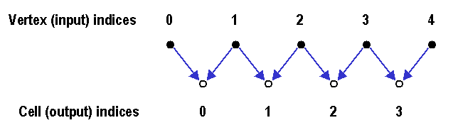
The required methods lowerExtent() and upperExtent() are very much like their Stencil counterparts. Because the output Field type of the FieldStencil has a different centering than the input Field type, however, care must be taken when interpreting these stencil widths. In this example, the input centering is Vert and the output centering is Cell. The value of lowerExtent(d) and upperExtent(d) are therefore 0 and 1 respectively, even though this is a centered-difference stencil, for which you might expect the lower extent to be -1 rather than zero.
To understand the values of lowerExtent(d) and upperExtent(d) for this cell-to-vertex stencil example, consider Figure 1, which is appropriate for any single value of the argument d.
The value returned by lowerExtent(d) is then the maximum positive integer offset from the element indexed by integer i in the input Field's index space along dimension d used in outputting the element indexed by integer i in the output Field's index space along dimension d. The (physical) domains of the input and output Fields along each dimension are of different lengths (because there is one more vertex than cell center along a dimension), so it is important to think carefully about what this implies about the stencil-width methods and the implementation of the operator() methods.
Applications can construct FieldStencil functors that are parameterized on functors such as the Div functor above, then invoke them via FieldStencil::operator() in the same way as was done with the Stencil<LaplaceStencil> functor in the Array Stencil example:
// Create the geometries, assuming RectilinearMesh object mesh:
typedef RectilinearMesh<Dim, Cartesian<Dim> > Mesh_t;
DiscreteGeometry<Vert, Mesh_t> geomv(mesh, GuardLayers<Dim>(1));
DiscreteGeometry<Cell, Mesh_t> geomc(mesh, GuardLayers<Dim>(1));

// Make the Fields (default EngineTag type):
Field<DiscreteGeometry<Vert, Mesh_t>, Vector<Dim> > vv(geomv);
Field<DiscreteGeometry<Cell, Mesh_t>, double > sc(geomc);

// Make the divergence FieldStencil object, using the Div class defined above:
typedef Div<Cell, DiscreteGeometry<Vert, Mesh_t>, Vector<Dim> > Div_t;
FieldStencil<Div_t> divVV2SC();

// Divergence, Vector/Vert-->Scalar/Cell
sc = divV2SC(vv);
Programmers may also find it convenient to create wrappers by defining global template functions which internally construct appropriate FieldStencil<class Stencil> objects, like the div() function described above.
Whenever POOMA encounters a data-parallel expression involving fields, boundary conditions may be applied. However, POOMA tries to ensure that these calculations are only done when absolutely necessary. Before evaluating an expression, POOMA asks each of the boundary conditions for each of the fields on the right-hand side of an assignment operator whether the source domain has been modified since the last time the boundary condition has been evaluated, and whether the domain for the data parallel expression touches the destination domain. The boundary condition is re-computed only if both of these are true. Otherwise, evaluation proceeds directly to the data-parallel expression.
Delaying evaluation in this way can forestall a lot of unnecessary calculation. The price for this is that programmers must be careful when writing scalar code, because scalar expression evaluation does not automatically trigger the update of field boundary conditions. To force calculation of all of a field's boundary conditions explicitly, an application must call the method Field::applyBoundaryConditions(). In particular:
In addition, boundary conditions are not automatically evaluated before a field is printed. Applications should therefore call applyBoundaryConditions() before output statements to ensure that the boundary values displayed are up to date.
POOMA includes a number of pre-built boundary conditions for use with fields and the supplied rectilinear meshes. For example, the following code sets the guard layers of a Dim-dimensional field f to zero:
for (int d = 0; d < 2 * Dim; d++)
{
  f.addBoundaryCondition(ZeroFaceBC(d));
}
All of the pre-built boundary conditions apply themselves to a particular face of the rectilinear computational domain. For each component direction, there is a high and a low face. For a Dim-dimensional field, faces are numbered consecutively from 0 to 2*Dim-1. The faces for each axis are numbered consecutively, with the low face having the lower (even) number. Thus, the coordinate direction and whether the face is the high or low face is calculated as follows:
int direction = face / 2;
bool isHigh   = (face & 1);
The high face in the Y direction therefore has a face index of 3 (second axis, second face).
The pre-built boundary conditions supported by POOMA are:
ConstantFaceBC<T> represents a Dirichlet boundary condition on a domain (i.e. one which keeps the value on that face constant). The constructor switch enforceConstantBoundary allows the boundary condition to enforce that the mesh-boundary value is constant, i.e. to determine whether the boundary condition writes into the guard layers, or into the actual physical domain. This affects only vertex-centered field values/components because the boundary is defined to be the last vertex. The T template parameter is the type of the constant value.
LinearExtrapolateFaceBC takes the values of the last two physical elements, and linearly extrapolates from the line through them out to all the guard elements. This is independent of centering. Like the other boundary conditions in this release of POOMA, it applies only to logically rectilinear domains.
NegReflectFaceBC represents an antisymmetric boundary condition on a logically rectilinear domain where the value on that face is assumed to be zero. As with the ConstantFaceBC boundary condition, the constructor switch enforceZeroBoundary allows the boundary condition to enforce that the boundary value is zero. This affects only vertex-centered field values/components because the boundary is defined to be the last vertex.
PeriodicFaceBC represents a periodic boundary condition in one direction of a logically rectilinear domain.
PosReflectFaceBC represents a symmetric boundary condition on a logically rectilinear domain; the face itself may take on any value. The constructor switch enforceZeroBoundary allows the boundary condition to enforce that the boundary value is zero. This affects only vertex-centered field values/components because the boundary is defined to be the last vertex.
ZeroFaceBC represents a zero Dirichlet boundary condition on a logically rectilinear domain. The constructor switch enforceZeroBoundary allows the boundary condition to enforce that the mesh-boundary value is zero. This affects only vertex-centered field values/components because the boundary is defined to be the last vertex.
Applications often need to apply different boundary conditions to different components of a Vector or Tensor field. In POOMA, this is accomplished using the ComponentBC adaptor, which works by taking a component view of the field and then applying the specified boundary condition to that view. Consider the example:
// Create the geometry.
typedef RectilinearCentering<D, VectorFaceRCTag<D> > Centering_t;
DiscreteGeometry<Centering_t, UniformRectilinearMesh<D> >
  geom(mesh, GuardLayers<D>(1));

// Make the field.
Field<DiscreteGeometry<Centering_t, UniformRectilinearMesh<D> >, Vector<D> >
  f(geom);

// Add componentwise boundary conditions.
typedef ComponentBC<1,NegReflectFaceBC> NegReflectFace_t;
typedef ComponentBC<1,PosReflectFaceBC> PosReflectFace_t;
for (int face = 0; face < 2 * D; face++)
{
  int direction = face / 2;
  for (int c = 0; c < D; c++)
  {
    if (c == direction)
      f.addBoundaryCondition(NegReflectFace_t(c, face));
    else
      f.addBoundaryCondition(PosReflectFace_t(c, face));
    }
}
This adds 2D2 boundary conditions for each of the D components at the high and low faces in each of the D coordinate directions. The ComponentBC class is templated on the number of indices (1 for Vectors and 2 for Tensors) and the boundary condition category (e.g., PosReflectFaceBC). The constructor arguments are the 1 or 2 indices specifying the components followed by the constructor arguments for the boundary condition.
It is often easiest for an application to set all of a field's boundary conditions at once. POOMA supports this by allowing boundary conditions to be initialized using a functor, as in:
f.addBoundaryConditions(AllZeroFaceBC());
This sets zero boundary conditions for all faces and components of the field f in a single statement. (Note the 's' at the end of the method name addBoundaryConditions()). The definition of the functor AllZeroFaceBC is simply:
class AllZeroFaceBC
{
public:
  AllZeroFaceBC(bool enforceZeroBoundary = false)
  : ezb_m(enforceZeroBoundary) { }

  template<class Geometry, class T, class EngineTag>
  void operator()(Field<Geometry, T, EngineTag> &f) const
  {
    for (int i = 0; i < 2 * Geometry::dimensions; i++)
    {
      f.addBoundaryCondition(ZeroFaceBC(i, ezb_m));
    }
  }
private:
  bool ezb_m;
};
Constructor arguments for the individual boundary conditions are specified when constructing the functor. The actual boundary conditions are added in the functor's operator() method, which is called internally by the field.
This release of POOMA predefines the functors listed below. Their effects can be inferred by comparing them with the boundary conditions given in the previous table.
In order to add a new type of boundary condition for POOMA, an application must define two classes: a boundary condition category, and the boundary condition itself. The boundary condition category class is the user interface for the boundary condition, and is simply a lightweight functor. (Classes like ConstantFaceBC<T> are boundary condition category classes of this kind.) For example, a boundary condition category for the following spatially-dependent two-dimensional boundary condition:
f(face) = 100 * x(face) * y(face)
could be written as:
class PositionFaceBC : public BCondCategory<PositionFaceBC>
{
public:
  PositionFaceBC(int face)
  : face_m(face)
  {}

  int face() const
  {
    return face_m;
  }

private:
  int face_m;
};
Notice that the class inherits from a version of BCondCategory templated on itself, but is otherwise quite straightforward.
The actual boundary condition is a specialization of the BCond class, which has the general template definition:
template<class Subject, class Category>
class BCond;
The Subject is the class of field that the boundary condition is to be applied to. POOMA needs to know this type exactly because it must be able to apply the boundary condition using PETE's data-parallel machinery.
To continue with the previous example, a specialization for the spatially-dependent boundary condition that is appropriate for two-dimensional multi-patch fields is:
typedef Field<
  DiscreteGeometry<Vert, UniformRectilinearMesh<2> >,
  double, MultiPatch<UniformTag, Brick> > FieldType_t;

template<>
class BCond<FieldType_t, PositionFaceBC> :
  public FieldBCondBase<FieldType_t>
{
public:
  // Constructor computes the destination domain
  BCond(const FieldType_t &f, const PositionFaceBC &bc)
  : FieldBCondBase<FieldType_t>(f, f.totalDomain())
  {
    int d = bc.face() / 2;
    int hiFace = bc.face() & 1;
    int layer;
    if (hiFace)
    {
      layer = destDomain()[d].last();
    }
    else
    {
      layer = destDomain()[d].first();
    }
    destDomain()[d] = Interval<1>(layer, layer);
  }

  void applyBoundaryCondition()
  {
    subject()(destDomain()) = 100.0 * subject().x(destDomain()).comp(0) *
      subject().x(destDomain()).comp(1);
  }

  BCond<FieldType_t, PositionFaceBC> *retarget(const FieldType_t &f) const
  {
    return new BCond<FieldType_t, PositionFaceBC>(f, bc_m);
  }
};
This could obviously be written more generally, but is sufficient to illustrate the concepts. Notice that this is a full specialization of the BCond template. Such specializations must inherit from the base class FieldBCondBase, which is templated on the field type.
The constructor for FieldBCondBase takes up to three arguments: the field, the initial value of the destination domain, and the initial value of the source domain. The last two domain arguments are optional. If they are not specified, the domains are initialized to be empty. The field argument can be subsequently accessed using the subject() member, the destination domain can be accessed using the destDomain() method, and the source domain can be accessed using the srcDomain() method.
The destination domain is the domain that fully bounds the region where the boundary condition is setting values. The source domain bounds the region where the boundary condition gets values to compute with. In this example, the destination domain is the single guard layer outside the physical domain for the specified face. There is no source domain because the destination values are not computed using other values. This is not the case with, for instance, the PeriodicFaceBC boundary condition, where periodicity is enforced by copying values from one place to another.
In many cases, the source and destination domains exactly define where values are read from, and where they are written. However, it is important to realize that POOMA treats these as bounding boxes. This means that for fields based on rectilinear meshes, the types of these domains will be Interval<Geometry::dimensions>. If a boundary condition doesn't write or read from domains specified by an Interval (e.g., a Range), this domain must be computed and stored specially.
For example, suppose an application had a boundary condition that set every other point in the guard layers. The destination domain member destDomain() would still return an Interval, since it represents a bounding box, not the actual domain. These two entities are the same for all of the boundary conditions that this release of POOMA contains; however, future versions may relax this constraint.
In addition to a constructor, a boundary value class must have a method called applyBoundaryCondition(), which must contain the code that actually evaluates the boundary condition, and a method called retarget(), which makes a new boundary condition using a different subject and the internal data of the current object. The example above uses straightforward data-parallel to syntax apply the boundary conditions. More sophisticated examples are included in the src/BConds directory in the release.
By default, POOMA associates boundary conditions with fields. This was done to allow automatic computation of boundary conditions and for compatibility with POOMA R1. An alternative approach is associating boundary conditions with operators. The source code below, taken from examples/Field/Laplace2, illustrates how this is done:
001  #include "Pooma/Fields.h"
002  #include "Utilities/Clock.h"
003
004  #include <iostream>
005
006  // Convenience typedefs.
007
008  typedef ConstField<
009    DiscreteGeometry<Vert, UniformRectilinearMesh<2> > > ConstFieldType_t;
010
011  typedef Field<
012    DiscreteGeometry<Vert, UniformRectilinearMesh<2> > > FieldType_t;
013
014  // The boundary condition.
015
016  class PositionFaceBC : public BCondCategory<PositionFaceBC>
017  {
018  public:
019
020    PositionFaceBC(int face) : face_m(face) { }
021
022    int face() const { return face_m; }
023
024  private:
025
026    int face_m;
027  };
028
029  template<>
030  class BCond<FieldType_t, PositionFaceBC>
031    : public FieldBCondBase<FieldType_t>
032  {
033  public:
034
035    BCond(const FieldType_t &f, const PositionFaceBC &bc)
036    : FieldBCondBase<FieldType_t>
037        (f, f.totalDomain()), bc_m(bc) { }
038
039    void applyBoundaryCondition()
040    {
041      int d = bc_m.face() / 2;
042      int hilo = bc_m.face() & 1;
043      int layer;
044      Interval<2> domain(subject().totalDomain());
045      if (hilo)
046        layer = domain[d].last();
047      else
048        layer = domain[d].first();
049
050      domain[d] = Interval<1>(layer, layer);
051      subject()(domain) = 100.0 * subject().x(domain).comp(0) *
052        subject().x(domain).comp(1);
053    }
054
055    BCond<FieldType_t, PositionFaceBC> *retarget(const FieldType_t &f) const
056    {
057      return new BCond<FieldType_t, PositionFaceBC>(f, bc_m);
058    }
059
060  private:
061
062    PositionFaceBC bc_m;
063  };
064
065  // The stencil.
066
067  class Laplacian
068  {
069  public:
070
071    typedef Vert OutputCentering_t;
072    typedef double OutputElement_t;
073
074    int lowerExtent(int) const { return 1; }
075    int upperExtent(int) const { return 1; }
076
077    template<class F>
078    inline OutputElement_t
079    operator()(const F &f, int i1, int i2) const
080    {
081      return 0.25 * (f(i1 + 1, i2) + f(i1 - 1, i2) +
082        f(i1, i2 + 1) + f(i1, i2 - 1));
083    }
084
085    template<class F>
086    static void applyBoundaryConditions(const F &f)
087    {
088      for (int i = 0; i < 4; i++)
089        {
090          BCondItem *bc = PositionFaceBC(i).create(f);
091          bc->applyBoundaryCondition();
092          delete bc;
093        }
094    }
095  };
096
097  void applyLaplacian(const FieldType_t &l, const FieldType_t &f)
098  {
099    Laplacian::applyBoundaryConditions(f);
100    l = FieldStencil<Laplacian>()(f);
101  }
102
103  int main(
104      int argc,
105      char *argv[]
106  ){
107      // Set up the library
108      Pooma::initialize(argc,argv);
109
110      // Create the physical domains:
111
112      // Set the dimensionality:
113      const int nVerts = 100;
114      Loc<2> center(nVerts / 2, nVerts / 2);
115      Interval<2> vertexDomain(nVerts, nVerts);
116
117      // Create the (uniform, logically rectilinear) mesh.
118      Vector<2> origin(1.0 / (nVerts + 1)), spacings(1.0 / (nVerts + 1));
119      typedef UniformRectilinearMesh<2> Mesh_t;
120      Mesh_t mesh(vertexDomain, origin, spacings);
121
122      // Create a geometry object with 1 guard layer to account for
123      // stencil width:
124      typedef DiscreteGeometry<Vert, UniformRectilinearMesh<2> > Geometry_t;
125      Geometry_t geom(mesh, GuardLayers<2>(1));
126
127      // Create the Fields:
128
129      // The voltage v(x,y) and a temporary vTemp(x,y):
130      FieldType_t v(geom), vTemp(geom);
131
132      // Start timing:
133      Pooma::Clock clock;
134      double start = clock.value();
135
136      // Load initial condition v(x,y) = 0:
137      v = 0.0;
138
139      // Perform the Jacobi iteration. We apply the Jacobi formula twice
140      // each loop:
141      double error = 1000;
142      int iteration = 0;
143      while (error > 1e-6)
144        {
145          iteration++;
146
147          applyLaplacian(vTemp, v);
148          applyLaplacian(v, vTemp);
149
150          // The analytic solution is v(x, y) = 100 * x * y so we can test the
151          // error:
152
153          // Make sure calculations are done prior to scalar calculations.
154          Pooma::blockAndEvaluate();
155
156          const double solution = v(center);
157          const double analytic = 100.0 * v.x(center)(0) * v.x(center)(1);
158          error = abs(solution - analytic);
159          if (iteration % 1000 == 0)
160            std::cout << "Iteration: " << iteration << "; "
161                << "Error: " << error << std::endl;
162        }
163
164      std::cout << "Wall clock time: " << clock.value() - start << std::endl;
165      std::cout << "Iteration: " << iteration << "; "
166                << "Error: " << error << std::endl;
167
168      Pooma::finalize();
169      return 0;
170  }
This is a simple Jacobi solver for Laplace's equation using the PositionFaceBC boundary condition discussed above. Lines 110-130 set up the mesh, the geometry, and the Brick-engine-based Field. Notice that we do not add any boundary conditions to this field, but we do reserve one layer of external guard layers (line 125). We then initialize the Field v and begin iterating. Since we need a temporary field to store the result of the Laplacian stencil, we can efficiently perform two applications of the stencil for each loop (lines 147 and 148). We know that the analytic solution of this problem is v(x, y) = 100 x y, so we can monitor and report the error in lines 156-161. Finally, we use the POOMA Clock class to monitor wall-clock time (lines 132-134 and 164).
The function applyLaplacian (lines 97-101) takes a Field to assign to and a Field to stencil as arguments. This is where the boundary conditions are applied, followed by the stencil. The Field stencil object Laplace is straightforward, except for the static function applyBoundaryConditions that, on the fly, creates boundary conditions for each face of the input field f and applies them.
Future versions of POOMA will better support this paradigm of associating boundary conditions with operators.
Fields are among the most important structures in physics, and
POOMA's Field classes are one of the things that make it more
than just another array package. While the facilities introduced in
this tutorial and the preceding one are more
complex than some other parts of POOMA, all of their complexity is
necessary in order to give applications programmers both expressive
power and high performance.
| [Prev] | [Home] | [Next] |